Uncertainty Quantification

Overview

At a high level, uncertainty quantification (UQ) or nondeterministic analysis is the process of (1) characterizing input uncertainties, (2) forward propagating these uncertainties through a computational model, and (3) performing statistical or interval assessments on the resulting responses. This process determines the effect of uncertainties and assumptions on model outputs or results. In Dakota, uncertainty quantification methods primarily focus on the forward propagation and analysis parts of the process (2 and 3), where probabilistic or interval information on parametric inputs are mapped through the computational model to assess statistics or intervals on outputs. For an overview of these approaches for engineering applications, consult [HM00]. Dakota also has emerging methods for inference or inverse UQ, such as Bayesian calibration. These methods help with (1) by inferring a statistical characterization of input parameters that is consistent with available observational data.

UQ is related to sensitivity analysis in that the common goal is to gain an understanding of how variations in the parameters affect the response functions of the engineering design problem. However, for UQ, some or all of the components of the parameter vector are considered to be uncertain as specified by particular probability distributions (e.g., normal, exponential, extreme value) or other uncertainty specifications. By assigning specific distributional structure to the inputs, distributional structure for the outputs (i.e, response statistics) can be inferred. This migrates from an analysis that is more qualitative in nature, in the case of sensitivity analysis, to an analysis that is more rigorously quantitative.

UQ methods can be distinguished by their ability to propagate aleatory or epistemic input uncertainty characterizations, where aleatory uncertainties are irreducible variabilities inherent in nature and epistemic uncertainties are reducible uncertainties resulting from a lack of knowledge.

For aleatory uncertainties, probabilistic methods are commonly used for computing response distribution statistics based on input probability distribution specifications. Conversely, for epistemic uncertainties, use of probability distributions is based on subjective prior knowledge rather than objective data, and we may alternatively explore nonprobabilistic methods based on interval specifications.

Summary of Dakota UQ Methods

Dakota contains capabilities for performing nondeterministic analysis with both types of input uncertainty. These UQ methods have been developed by Sandia Labs, in conjunction with collaborators in academia [EAP+07, GRH99, GS91, TSE10].

The aleatory UQ methods in Dakota include various sampling-based approaches (e.g., Monte Carlo and Latin Hypercube sampling), local and global reliability methods, and stochastic expansion (polynomial chaos expansions, stochastic collocation, and functional tensor train) approaches. The epistemic UQ methods include local and global interval analysis and Dempster-Shafer evidence theory. These are summarized below and then described in more depth in subsequent sections of this chapter. Dakota additionally supports mixed aleatory/epistemic UQ via interval-valued probability, second-order probability, and Dempster-Shafer theory of evidence. These involve advanced model recursions and are described in Mixed Aleatory-Epistemic UQ.

LHS (Latin Hypercube Sampling): This package provides both Monte Carlo (random) sampling and Latin Hypercube sampling methods, which can be used with probabilistic variables in Dakota that have the following distributions: normal, lognormal, uniform, loguniform, triangular, exponential, beta, gamma, gumbel, frechet, weibull, poisson, binomial, negative binomial, geometric, hypergeometric, and user-supplied histograms. In addition, LHS accounts for correlations among the variables [IS84], which can be used to accommodate a user-supplied correlation matrix or to minimize correlation when a correlation matrix is not supplied. In addition to a standard sampling study, we support the capability to perform “incremental” LHS, where a user can specify an initial LHS study of N samples, and then re-run an additional incremental study which will double the number of samples (to 2N, with the first N being carried from the initial study). The full incremental sample of size 2N is also a Latin Hypercube, with proper stratification and correlation. Statistics for each increment are reported separately at the end of the study.

Reliability Methods: This suite of methods includes both local and global reliability methods. Local methods include first- and second-order versions of the Mean Value method (MVFOSM and MVSOSM) and a variety of most probable point (MPP) search methods, including the Advanced Mean Value method (AMV and AMV\(^2\)), the iterated Advanced Mean Value method (AMV+ and AMV\(^2\)+), the Two-point Adaptive Nonlinearity Approximation method (TANA-3), and the traditional First Order and Second Order Reliability Methods (FORM and SORM) [HM00]. The MPP search methods may be used in forward (Reliability Index Approach (RIA)) or inverse (Performance Measure Approach (PMA)) modes, as dictated by the type of level mappings. Each of the MPP search techniques solve local optimization problems in order to locate the MPP, which is then used as the point about which approximate probabilities are integrated (using first- or second-order integrations in combination with refinements based on importance sampling). Global reliability methods are designed to handle nonsmooth and multimodal failure surfaces, by creating global approximations based on Gaussian process models. They accurately resolve a particular contour of a response function and then estimate probabilities using multimodal adaptive importance sampling.

Stochastic Expansion Methods: Theoretical development of these techniques mirrors that of deterministic finite element analysis utilizing the notions of projection, orthogonality, and weak convergence [GRH99], [GS91].

Rather than focusing on estimating specific statistics (e.g., failure probability), they form an approximation to the functional relationship between response functions and their random inputs, which provides a more complete uncertainty representation for use in more advanced contexts, such as coupled multi-code simulations. Expansion methods include polynomial chaos expansions (PCE), which expand in a basis of multivariate orthogonal polynomials (e.g., Hermite, Legendre) that are tailored to representing particular input probability distributions (e.g., normal, uniform); stochastic collocation (SC), which expand in a basis of multivariate interpolation polynomials (e.g., Lagrange); and functional tensor train (FTT), which leverages concepts from data compression to expand using low rank products of polynomial cores. For PCE, expansion coefficients may be evaluated using a spectral projection approach (based on sampling, tensor-product quadrature, Smolyak sparse grid, or cubature methods for numerical integration) or a regression approach (least squares or compressive sensing). For SC, interpolants are formed over tensor-product or sparse grids and may be local or global, value-based or gradient-enhanced, and nodal or hierarchical. In global value-based cases (Lagrange polynomials), the barycentric formulation is used [BT04, Hig04, Kli05] to improve numerical efficiency and stability. For FTT, regression via regularized nonlinear least squares is employed for recovering low rank coefficients, and cross-validation schemes are available to determine the best rank and polynomial basis order settings. Each of these methods provide analytic response moments and variance-based metrics; however, PDFs and CDF/CCDF mappings are computed numerically by sampling on the expansion.

Importance Sampling: Importance sampling is a method that allows one to estimate statistical quantities such as failure probabilities in a way that is more efficient than Monte Carlo sampling. The core idea in importance sampling is that one generates samples that are preferentially placed in important regions of the space (e.g. in or near the failure region or user-defined region of interest), then appropriately weights the samples to obtain an unbiased estimate of the failure probability.

Adaptive Sampling: The goal in performing adaptive sampling is to construct a surrogate model that can be used as an accurate predictor of an expensive simulation. The aim is to build a surrogate that minimizes the error over the entire domain of interest using as little data as possible from the expensive simulation. The adaptive sampling methods start with an initial LHS sample, and then adaptively choose samples that optimize a particular criteria. For example, if a set of additional possible sample points are generated, one criteria is to pick the next sample point as the point which maximizes the minimum distance to the existing points (maximin). Another criteria is to pick the sample point where the surrogate indicates the most uncertainty in its prediction.

Recently, Dakota added a new method to assess failure probabilities based on ideas from computational geometry. Part of the idea underpinning this method is the idea of throwing “darts” which are higher dimensional objects than sample points (e.g. lines, planes, etc.) The POF (Probability-of-Failure) darts method uses these objects to estimate failure probabilities.

Interval Analysis: Interval analysis is often used to model epistemic uncertainty. In interval analysis, one assumes that nothing is known about an epistemic uncertain variable except that its value lies somewhere within an interval. In this situation, it is NOT assumed that the value has a uniform probability of occurring within the interval. Instead, the interpretation is that any value within the interval is a possible value or a potential realization of that variable. In interval analysis, the uncertainty quantification problem is one of determining the resulting bounds on the output (defining the output interval) given interval bounds on the inputs. Again, any output response that falls within the output interval is a possible output with no frequency information assigned to it.

We have the capability to perform interval analysis using either global or local methods. In the global approach, one uses either a global optimization method (based on a Gaussian process surrogate model) or a sampling method to assess the bounds. The local method uses gradient information in a derivative-based optimization approach, using either SQP (sequential quadratic programming) or a NIP (nonlinear interior point) method to obtain bounds.

Dempster-Shafer Theory of Evidence: The objective of evidence theory is to model the effects of epistemic uncertainties. Epistemic uncertainty refers to the situation where one does not know enough to specify a probability distribution on a variable. Sometimes epistemic uncertainty is referred to as subjective, reducible, or lack of knowledge uncertainty. In contrast, aleatory uncertainty refers to the situation where one does have enough information to specify a probability distribution. In Dempster-Shafer theory of evidence, the uncertain input variables are modeled as sets of intervals. The user assigns a basic probability assignment (BPA) to each interval, indicating how likely it is that the uncertain input falls within the interval. The intervals may be overlapping, contiguous, or have gaps. The intervals and their associated BPAs are then propagated through the simulation to obtain cumulative distribution functions on belief and plausibility. Belief is the lower bound on a probability estimate that is consistent with the evidence, and plausibility is the upper bound on a probability estimate that is consistent with the evidence. In addition to the full evidence theory structure, we have a simplified capability for users wanting to perform pure interval analysis (e.g. what is the interval on the output given intervals on the input) using either global or local optimization methods. Interval analysis is often used to model epistemic variables in nested analyses, where probability theory is used to model aleatory variables.

Bayesian Calibration: In Bayesian calibration, uncertain input parameters are initially characterized by a “prior” distribution. A Bayesian calibration approach uses experimental data together with a likelihood function, which describes how well a realization of the parameters is supported by the data, to update this prior knowledge. The process yields a posterior distribution of the parameters most consistent with the data, such that running the model at samples from the posterior yields results consistent with the observational data.

Variables and Responses for UQ

UQ methods that perform a forward uncertainty propagation map probability or interval information for input parameters into probability or interval information for output response functions. The \(m\) functions in the Dakota response data set are interpreted as \(m\) general response functions by the Dakota methods (with no specific interpretation of the functions as for optimization and least squares).

Within the variables specification, uncertain variable descriptions are employed to define the random variable distributions (refer to Uncertain Variables). For Bayesian inference methods, these uncertain variable properties characterize the prior distribution to be updated and constrained by the observational data. As enumerated in Uncertain Variables, uncertain variables types are categorized as either aleatory or epistemic and as either continuous or discrete, where discrete types include integer ranges, integer sets, string sets, and real sets. The continuous aleatory distribution types include: normal (Gaussian), lognormal, uniform, loguniform, triangular, exponential, beta, gamma, gumbel, frechet, weibull, and histogram bin. The discrete aleatory distribution types include: poisson, binomial, negative binomial, geometric, hypergeometric, and discrete histograms for integers, strings, and reals. The epistemic distribution types include continuous intervals, discrete integer ranges, and discrete sets for integers, strings, and reals. While many of the epistemic types appear similar to aleatory counterparts, a key difference is that the latter requires probabilities for each value within a range or set, whereas the former will use, at most, a subjective belief specification.

When gradient and/or Hessian information is used in an uncertainty assessment, derivative components are normally computed with respect to the active continuous variables, which could be aleatory uncertain, epistemic uncertain, aleatory and epistemic uncertain, or all continuous variables, depending on the active view (see Management of Mixed Variables by Method).

Sampling Methods

Sampling techniques are selected using the sampling method selection. This method generates sets of samples according to the probability distributions of the uncertain variables and maps them into corresponding sets of response functions, where the number of samples is specified by the samples integer specification. Means, standard deviations, coefficients of variation (COVs), and 95% confidence intervals are computed for the response functions. Probabilities and reliabilities may be computed for response_levels specifications, and response levels may be computed for either probability_levels or reliability_levels specifications.

Currently, traditional Monte Carlo (MC) and Latin hypercube sampling (LHS) are supported by Dakota and are chosen by specifying sample_type as random or lhs. In Monte Carlo sampling, the samples are selected randomly according to the user-specified probability distributions. Latin hypercube sampling is a stratified sampling technique for which the range of each uncertain variable is divided into \(N_{s}\) segments of equal probability, where \(N_{s}\) is the number of samples requested. The relative lengths of the segments are determined by the nature of the specified probability distribution (e.g., uniform has segments of equal width, normal has small segments near the mean and larger segments in the tails). For each of the uncertain variables, a sample is selected randomly from each of these equal probability segments. These \(N_{s}\) values for each of the individual parameters are then combined in a shuffling operation to create a set of \(N_{s}\) parameter vectors with a specified correlation structure. A feature of the resulting sample set is that every row and column in the hypercube of partitions has exactly one sample. Since the total number of samples is exactly equal to the number of partitions used for each uncertain variable, an arbitrary number of desired samples is easily accommodated (as compared to less flexible approaches in which the total number of samples is a product or exponential function of the number of intervals for each variable, i.e., many classical design of experiments methods).

Advantages of sampling-based methods include their relatively simple implementation and their independence from the scientific disciplines involved in the analysis. The main drawback of these techniques is the large number of function evaluations needed to generate converged statistics, which can render such an analysis computationally very expensive, if not intractable, for real-world engineering applications. LHS techniques, in general, require fewer samples than traditional Monte Carlo for the same accuracy in statistics, but they still can be prohibitively expensive. For further information on the method and its relationship to other sampling techniques, one is referred to the works by McKay, et al. [MBC79], Iman and Shortencarier [IS84], and Helton and Davis [HD00]. Note that under certain separability conditions associated with the function to be sampled, Latin hypercube sampling provides a more accurate estimate of the mean value than does random sampling. That is, given an equal number of samples, the LHS estimate of the mean will have less variance than the mean value obtained through random sampling.

Fig. 39 demonstrates Latin hypercube sampling on a two-variable parameter space. Here, the range of both parameters, \(x_1\) and \(x_2\), is \([0,1]\). Also, for this example both \(x_1\) and \(x_2\) have uniform statistical distributions. For Latin hypercube sampling, the range of each parameter is divided into \(p\) “bins” of equal probability. For parameters with uniform distributions, this corresponds to partitions of equal size. For \(n\) design parameters, this partitioning yields a total of \(p^{n}\) bins in the parameter space. Next, \(p\) samples are randomly selected in the parameter space, with the following restrictions: (a) each sample is randomly placed inside a bin, and (b) for all one-dimensional projections of the \(p\) samples and bins, there will be one and only one sample in each bin. In a two-dimensional example such as that shown in Fig. 39, these LHS rules guarantee that only one bin can be selected in each row and column. For \(p=4\), there are four partitions in both \(x_1\) and \(x_2\). This gives a total of 16 bins, of which four will be chosen according to the criteria described above. Note that there is more than one possible arrangement of bins that meet the LHS criteria. The dots in Fig. 39 represent the four sample sites in this example, where each sample is randomly located in its bin. There is no restriction on the number of bins in the range of each parameter, however, all parameters must have the same number of bins.

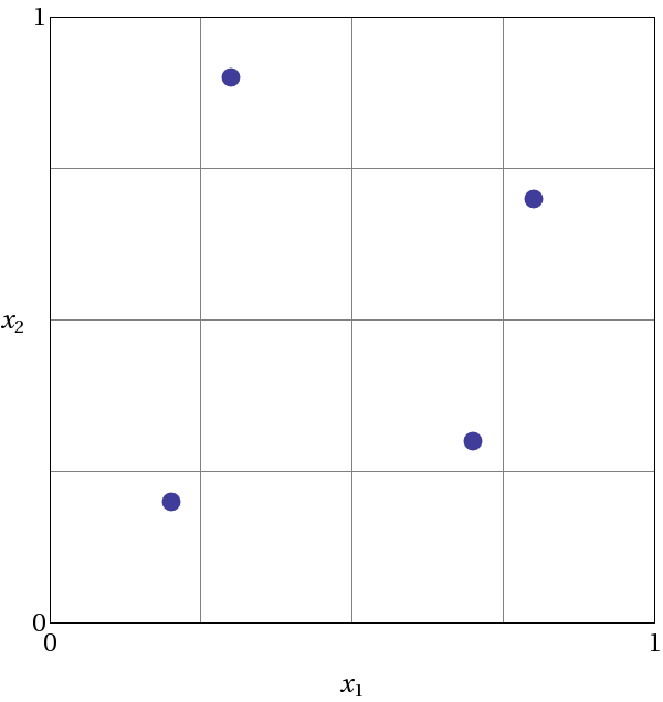
An example of Latin hypercube sampling with four bins in design parameters :math:`x_1` and :math:`x_2`. The dots are the sample sites. — Fig. 39 An example of Latin hypercube sampling with four bins in design parameters \(x_1\) and \(x_2\). The dots are the sample sites.

The actual algorithm for generating Latin hypercube samples is more complex than indicated by the description given above. For example, the Latin hypercube sampling method implemented in the LHS code [SW04] takes into account a user-specified correlation structure when selecting the sample sites. For more details on the implementation of the LHS algorithm, see Reference [SW04].

In addition to Monte Carlo vs. LHS design choices, Dakota sampling methods support options for incrementally-refined designs, generation of approximately determinant-optimal (D-optimal) designs, and selection of sample sizes to satisfy Wilks’ criteria.

Uncertainty Quantification Example using Sampling Methods

The input file in Listing 29 demonstrates the use of Latin hypercube Monte Carlo sampling for assessing probability of failure as measured by specified response levels. The two-variable Textbook example problem (see Textbook) will be used to demonstrate the application of sampling methods for uncertainty quantification where it is assumed that \(x_1\) and \(x_2\) are uniform uncertain variables on the interval \([0,1]\).

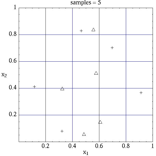
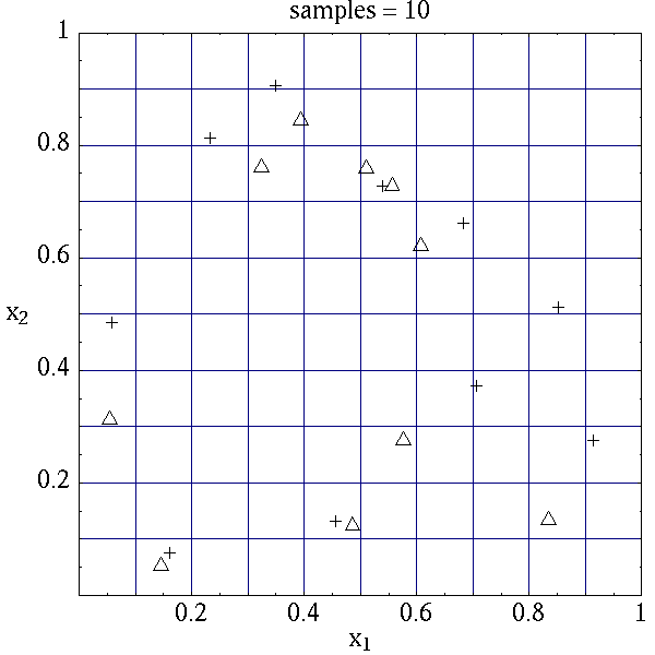
The number of samples to perform is controlled with the samples specification, the type of sampling algorithm to use is controlled with the sample_type specification, the levels used for computing statistics on the response functions is specified with the response_levels input, and the seed specification controls the sequence of the pseudo-random numbers generated by the sampling algorithms. The input samples generated are shown in Table 7 for the case where samples = 5 and samples = 10 for both random (\(\triangle\)) and lhs (\(+\)) sample types.

Listing 29 Dakota input file for UQ example using LHS – see dakota/share/dakota/examples/users/textbook_uq_sampling.in

# Dakota Input File: textbook_uq_sampling.in
environment
  tabular_data
    tabular_data_file = 'textbook_uq_sampling.dat'
  top_method_pointer = 'UQ'

method
  id_method = 'UQ'
  sampling
    sample_type lhs
    samples = 10
    seed = 98765
    response_levels = 0.1 0.2 0.6
                      0.1 0.2 0.6
                      0.1 0.2 0.6
    distribution cumulative

variables
  uniform_uncertain = 2
    lower_bounds =  0.   0.
    upper_bounds =  1.   1.
    descriptors  = 'x1' 'x2'

interface
  id_interface = 'I1'
  analysis_drivers = 'text_book'
    fork
  asynchronous evaluation_concurrency = 5

responses
  response_functions = 3
  no_gradients
  no_hessians

Table 7 Distribution of input sample points for random (\(\triangle\)) and lhs (\(+\)) sampling for (a) samples=5 and (b) samples=10.

Latin hypercube sampling ensures full coverage of the range of the input variables, which is often a problem with Monte Carlo sampling when the number of samples is small. In the case of samples = 5, poor stratification is evident in \(x_1\) as four out of the five Monte Carlo samples are clustered in the range \(0.35 < x_1 < 0.55\), and the regions \(x_1 < 0.3\) and \(0.6 < x_1 < 0.9\) are completely missed. For the case where samples = 10, some clustering in the Monte Carlo samples is again evident with 4 samples in the range \(0.5 < x_1 < 0.55\). In both cases, the stratification with LHS is superior.

The response function statistics returned by Dakota are shown in Listing 30. The first block of output specifies the response sample means, sample standard deviations, and skewness and kurtosis. The second block of output displays confidence intervals on the means and standard deviations of the responses. The third block defines Probability Density Function (PDF) histograms of the samples: the histogram bins are defined by the lower and upper values of the bin and the corresponding density for that bin. Note that these bin endpoints correspond to the response_levels and/or probability_levels defined by the user in the Dakota input file. If there are just a few levels, these histograms may be coarse. Dakota does not do anything to optimize the bin size or spacing. Finally, the last section of the output defines the Cumulative Distribution Function (CDF) pairs. In this case, distribution cumulative was specified for the response functions, and Dakota presents the probability levels corresponding to the specified response levels (response_levels) that were set. The default compute probabilities was used. Alternatively, Dakota could have provided CCDF pairings, reliability levels corresponding to prescribed response levels, or response levels corresponding to prescribed probability or reliability levels.

Listing 30 Dakota response function statistics from UQ sampling example.

Statistics based on 10 samples:

Sample moment statistics for each response function:
                            Mean           Std Dev          Skewness          Kurtosis
 response_fn_1  3.8383990322e-01  4.0281539886e-01  1.2404952971e+00  6.5529797327e-01
 response_fn_2  7.4798705803e-02  3.4686110941e-01  4.5716015887e-01 -5.8418924529e-01
 response_fn_3  7.0946176558e-02  3.4153246532e-01  5.2851897926e-01 -8.2527332042e-01

95% confidence intervals for each response function:
                    LowerCI_Mean      UpperCI_Mean    LowerCI_StdDev    UpperCI_StdDev
 response_fn_1  9.5683125821e-02  6.7199668063e-01  2.7707061315e-01  7.3538389383e-01
 response_fn_2 -1.7333078422e-01  3.2292819583e-01  2.3858328290e-01  6.3323317325e-01
 response_fn_3 -1.7337143113e-01  3.1526378424e-01  2.3491805390e-01  6.2350514636e-01

Probability Density Function (PDF) histograms for each response function:
PDF for response_fn_1:
          Bin Lower          Bin Upper      Density Value
          ---------          ---------      -------------
   2.3066424677e-02   1.0000000000e-01   3.8994678038e+00
   1.0000000000e-01   2.0000000000e-01   2.0000000000e+00
   2.0000000000e-01   6.0000000000e-01   5.0000000000e-01
   6.0000000000e-01   1.2250968624e+00   4.7992562123e-01
PDF for response_fn_2:
          Bin Lower          Bin Upper      Density Value
          ---------          ---------      -------------
  -3.5261164651e-01   1.0000000000e-01   1.1046998102e+00
   1.0000000000e-01   2.0000000000e-01   2.0000000000e+00
   2.0000000000e-01   6.0000000000e-01   5.0000000000e-01
   6.0000000000e-01   6.9844576220e-01   1.0157877573e+00
PDF for response_fn_3:
          Bin Lower          Bin Upper      Density Value
          ---------          ---------      -------------
  -3.8118095128e-01   1.0000000000e-01   1.2469321539e+00
   1.0000000000e-01   2.0000000000e-01   0.0000000000e+00
   2.0000000000e-01   6.0000000000e-01   7.5000000000e-01
   6.0000000000e-01   6.4526450977e-01   2.2092363423e+00

Level mappings for each response function:
Cumulative Distribution Function (CDF) for response_fn_1:
     Response Level  Probability Level  Reliability Index  General Rel Index
     --------------  -----------------  -----------------  -----------------
   1.0000000000e-01   3.0000000000e-01
   2.0000000000e-01   5.0000000000e-01
   6.0000000000e-01   7.0000000000e-01
Cumulative Distribution Function (CDF) for response_fn_2:
     Response Level  Probability Level  Reliability Index  General Rel Index
     --------------  -----------------  -----------------  -----------------
   1.0000000000e-01   5.0000000000e-01
   2.0000000000e-01   7.0000000000e-01
   6.0000000000e-01   9.0000000000e-01
Cumulative Distribution Function (CDF) for response_fn_3:
     Response Level  Probability Level  Reliability Index  General Rel Index
     --------------  -----------------  -----------------  -----------------
   1.0000000000e-01   6.0000000000e-01
   2.0000000000e-01   6.0000000000e-01
   6.0000000000e-01   9.0000000000e-01

In addition to obtaining statistical summary information of the type shown in Listing 30, the results of LHS sampling also include correlations.

Four types of correlations are returned in the output: simple and partial “raw” correlations, and simple and partial “rank” correlations. The raw correlations refer to correlations performed on the actual input and output data. Rank correlations refer to correlations performed on the ranks of the data. Ranks are obtained by replacing the actual data by the ranked values, which are obtained by ordering the data in ascending order. For example, the smallest value in a set of input samples would be given a rank 1, the next smallest value a rank 2, etc. Rank correlations are useful when some of the inputs and outputs differ greatly in magnitude: then it is easier to compare if the smallest ranked input sample is correlated with the smallest ranked output, for example.

Correlations are always calculated between two sets of sample data. One can calculate correlation coefficients between two input variables, between an input and an output variable (probably the most useful), or between two output variables. The simple correlation coefficients presented in the output tables are Pearson’s correlation coefficient, which is defined for two variables \(x\) and \(y\) as: \(\mathtt{Corr}(x,y) = \frac{\sum_{i}(x_{i}-\bar{x})(y_{i}-\bar{y})} {\sqrt{\sum_{i}(x_{i}-\bar{x})^2\sum_{i}(y_{i}-\bar{y})^2}}\). Partial correlation coefficients are similar to simple correlations, but a partial correlation coefficient between two variables measures their correlation while adjusting for the effects of the other variables. For example, say one has a problem with two inputs and one output; and the two inputs are highly correlated. Then the correlation of the second input and the output may be very low after accounting for the effect of the first input. The rank correlations in Dakota are obtained using Spearman’s rank correlation. Spearman’s rank is the same as the Pearson correlation coefficient except that it is calculated on the rank data.

Listing 31 shows an example of the correlation output provided by Dakota for the input file in Listing 29. Note that these correlations are presently only available when one specifies lhs as the sampling method under sampling. Also note that the simple and partial correlations should be similar in most cases (in terms of values of correlation coefficients). This is because we use a default “restricted pairing” method in the LHS routine which forces near-zero correlation amongst uncorrelated inputs.

Listing 31 Correlation results using LHS Sampling.

Simple Correlation Matrix between input and output:
                       x1           x2 response_fn_1 response_fn_2 response_fn_3
          x1  1.00000e+00
          x2 -7.22482e-02  1.00000e+00
response_fn_1 -7.04965e-01 -6.27351e-01  1.00000e+00
response_fn_2  8.61628e-01 -5.31298e-01 -2.60486e-01  1.00000e+00
response_fn_3 -5.83075e-01  8.33989e-01 -1.23374e-01 -8.92771e-01  1.00000e+00

Partial Correlation Matrix between input and output:
             response_fn_1 response_fn_2 response_fn_3
          x1 -9.65994e-01  9.74285e-01 -9.49997e-01
          x2 -9.58854e-01 -9.26578e-01  9.77252e-01

Simple Rank Correlation Matrix between input and output:
                       x1           x2 response_fn_1 response_fn_2 response_fn_3
          x1  1.00000e+00
          x2 -6.66667e-02  1.00000e+00
response_fn_1 -6.60606e-01 -5.27273e-01  1.00000e+00
response_fn_2  8.18182e-01 -6.00000e-01 -2.36364e-01  1.00000e+00
response_fn_3 -6.24242e-01  7.93939e-01 -5.45455e-02 -9.27273e-01  1.00000e+00

Partial Rank Correlation Matrix between input and output:
             response_fn_1 response_fn_2 response_fn_3
          x1 -8.20657e-01  9.74896e-01 -9.41760e-01
          x2 -7.62704e-01 -9.50799e-01  9.65145e-01

Finally, note that the LHS package can be used for design of experiments over design and state variables by including an active view override in the variables specification section of the Dakota input file (see Active Variables View). Then, instead of iterating on only the uncertain variables, the LHS package will sample over all of the active variables. In the active all view, continuous design and continuous state variables are treated as having uniform probability distributions within their upper and lower bounds, discrete design and state variables are sampled uniformly from within their sets or ranges, and any uncertain variables are sampled within their specified probability distributions.

Incremental Sampling

In many situations, one may run an initial sample set and then need to perform further sampling to get better estimates of the mean, variance, and percentiles, and to obtain more comprehensive sample coverage. We call this capability incremental sampling. Typically, a Dakota restart file (dakota.rst) would be available from the original sample, so only the newly generated samples would need to be evaluated. Incremental sampling supports continuous uncertain variables and discrete uncertain variables such as discrete distributions (e.g. binomial, Poisson, etc.) as well as histogram variables and uncertain set types.

There are two cases, incremental random and incremental Latin hypercube sampling, with incremental LHS being the most common. One major advantage of LHS incremental sampling is that it maintains the stratification and correlation structure of the original LHS sample. That is, if one generated two independent LHS samples and simply merged them, the calculation of the accuracy of statistical measures such as the mean and the variance would be slightly incorrect. However, in the incremental case, the full sample (double the original size) is a Latin Hypercube sample itself and statistical measures and their accuracy can be properly calculated. The incremental sampling capability is most useful when one is starting off with very small samples. Once the sample size is more than a few hundred, the benefit of incremental sampling diminishes.

Incremental random sampling: With incremental random sampling, the original sample set with \(N1\) samples must be generated using sample_type = random and samples = N1. Then, the user can duplicate the Dakota input file and add refinement_samples = N2 with the number of new samples \(N2\) to be added. Random incremental sampling does not require a doubling of samples each time. Thus, the user can specify any number of refinement_samples (from an additional one sample to a large integer).

For example, if the first sample has 50 samples, and 10 more samples are desired, the second Dakota run should specify samples = 50, refinement_samples = 10. In this situation, only 10 new samples will be generated, and the final statistics will be reported at the end of the study both for the initial 50 samples and for the full sample of 60. The command line syntax for running the second sample is dakota -i input60.in -r dakota.50.rst where input60.in is the input file with the refinement samples specification and dakota.50.rst is the restart file containing the initial 50 samples. Note that if the restart file has a different name, that is fine; the correct restart file name should be used.

This process can be repeated if desired,arbitrarily extending the total sample size each time, e.g, samples = 50, refinement_samples = 10 3 73 102.
Incremental Latin hypercube sampling: With incremental LHS sampling, the original sample set with \(N1\) samples must be generated using sample_type = lhs and samples = N1. Then, the user can duplicate the Dakota input file and add refinement_samples = N1. The sample size must double each time, so the first set of refinement samples must be the same size as the initial set. That is, if one starts with a very small sample size of 10, then one can use the incremental sampling capability to generate sample sizes of 20, 40, 80, etc.

For example, if the first sample has 50 samples, in the second Dakota run, the number of refinement samples should be set to 50 for a total of 100. In this situation, only 50 new samples will be generated, and at the end of the study final statistics will be reported both for the initial 50 samples and for the full sample of 100. The command line syntax for running the second sample is dakota -i input100.in -r dakota.50.rst, where input100.in is the input file with the incremental sampling specification and dakota.50.rst is the restart file containing the initial 50 samples. Note that if the restart file has a different name, that is fine; the correct restart file name should be used.

This process can be repeated if desired, doubling the total sample size each time, e.g, samples = 50, refinement_samples = 50 100 200 400.

Principal Component Analysis

As of Dakota 6.3, we added a capability to perform Principal Component Analysis on field response data when using LHS sampling. Principal components analysis (PCA) is a data reduction method and allows one to express an ensemble of field data with a set of principal components responsible for the spread of that data.

Dakota can calculate the principal components of the response matrix of N samples * L responses (the field response of length L) using the keyword principal_components. The Dakota implementation is under active development: the PCA capability may ultimately be specified elsewhere or used in different ways. For now, it is performed as a post-processing analysis based on a set of Latin Hypercube samples.

If the user specifies LHS sampling with field data responses and also specifies principal_components, Dakota will calculate the principal components by calculating the eigenvalues and eigenvectors of a centered data matrix. Further, if the user specifies percent_variance_explained = 0.99, the number of components that accounts for at least 99 percent of the variance in the responses will be retained. The default for this percentage is 0.95. In many applications, only a few principal components explain the majority of the variance, resulting in significant data reduction. The principal components are written to a file princ_comp.txt. Dakota also uses the principal components to create a surrogate model by representing the overall response as weighted sum of M principal components, where the weights will be determined by Gaussian processes which are a function of the input uncertain variables. This reduced form then can be used for sensitivity analysis, calibration, etc.

Wilks-based Sample Sizes

Most of the sampling methods require the user to specify the number of samples in advance. However, if one specifies random sampling, one can use an approach developed by Wilks:cite:p:Wilks to determine the number of samples that ensures a particular confidence level in a percentile of interest. The Wilks method of computing the number of samples to execute for a random sampling study is based on order statistics, eg considering the outputs ordered from smallest to largest [NW04, Wil41]. Given a probability_level, \(\alpha\), and confidence_level, \(\beta\), the Wilks calculation determines the minimum number of samples required such that there is \((\beta*100)\)% confidence that the \((\alpha*100)\)%-ile of the uncertain distribution on model output will fall below the actual \((\alpha*100)\)%-ile given by the sample. To be more specific, if we wish to calculate the \(95\%\) confidence limit on the \(95^{th}\) percentile, Wilks indicates that 59 samples are needed. If we order the responses and take the largest one, that value defines a tolerance limit on the 95th percentile: we have a situation where \(95\%\) of the time, the \(95^{th}\) percentile will fall at or below that sampled value. This represents a one_sided_upper treatment applicable to the largest output value. This treatment can be reversed to apply to the lowest output value by using the one_sided_lower option, and further expansion to include an interval containing both the smallest and the largest output values in the statistical statement can be specified via the two_sided option. Additional generalization to higher order statistics, eg a statement applied to the N largest outputs (one_sided_upper) or the N smallest and N largest outputs (two_sided), can be specified using the order option along with value N.

Double Sided Tolerance Interval Equivalent Normal Distribution

Tolerance Intervals (TIs) are a simple way to approximately account for the epistemic sampling uncertainty introduced from finite samples of a random variable. TIs are parameterized by two user-prescribed levels: one for the desired “coverage” proportion of a distribution and one for the desired degree of statistical “confidence” in covering or bounding at least that proportion. For instance, a \(95\%\) coverage / \(90\%\) confidence TI (\(95\%\)/\(90\%\) TI, \(95\)/\(90\) TI, or \(0.95\)/\(0.90\) TI) prescribes lower and upper values of a range said to have at least \(90\%\) odds that it covers or spans \(95\%\) of the “true” probability distribution from which the random samples were drawn, if they were drawn from a Normal distribution [JR20].

Reliability Methods

Reliability methods provide an alternative approach to uncertainty quantification which can be less computationally demanding than sampling techniques. Reliability methods for uncertainty quantification are based on probabilistic approaches that compute approximate response function distribution statistics based on specified uncertain variable distributions. These response statistics include response mean, response standard deviation, and cumulative or complementary cumulative distribution functions (CDF/CCDF). These methods are often more efficient at computing statistics in the tails of the response distributions (events with low probability) than sampling based approaches since the number of samples required to resolve a low probability can be prohibitive.

The methods all answer the fundamental question: “Given a set of uncertain input variables, \(\mathbf{X}\), and a scalar response function, \(g\), what is the probability that the response function is below or above a certain level, \(\bar{z}\)?” The former can be written as \(P[g(\mathbf{X}) \le \bar{z}] = \mathit{F}_{g}(\bar{z})\) where \(\mathit{F}_{g}(\bar{z})\) is the cumulative distribution function (CDF) of the uncertain response \(g(\mathbf{X})\) over a set of response levels. The latter can be written as \(P[g(\mathbf{X}) > \bar{z}]\) and defines the complementary cumulative distribution function (CCDF).

This probability calculation involves a multi-dimensional integral over an irregularly shaped domain of interest, \(\mathbf{D}\), where \(g(\mathbf{X}) < z\) as displayed in Fig. 40 for the case of two variables. The reliability methods all involve the transformation of the user-specified uncertain variables, \(\mathbf{X}\), with probability density function, \(p(x_1,x_2)\), which can be non-normal and correlated, to a space of independent Gaussian random variables, \(\mathbf{u}\), possessing a mean value of zero and unit variance (i.e., standard normal variables). The region of interest, \(\mathbf{D}\), is also mapped to the transformed space to yield, \(\mathbf{D_{u}}\) , where \(g(\mathbf{U}) < z\) as shown in Fig. 41. The Nataf transformation [DKL86], which is identical to the Rosenblatt transformation [Ros52] in the case of independent random variables, is used in Dakota to accomplish this mapping. This transformation is performed to make the probability calculation more tractable. In the transformed space, probability contours are circular in nature as shown in Fig. 41 unlike in the original uncertain variable space, Fig. 40. Also, the multi-dimensional integrals can be approximated by simple functions of a single parameter, \(\beta\), called the reliability index. \(\beta\) is the minimum Euclidean distance from the origin in the transformed space to the response surface. This point is also known as the most probable point (MPP) of failure. Note, however, the methodology is equally applicable for generic functions, not simply those corresponding to failure criteria; this nomenclature is due to the origin of these methods within the disciplines of structural safety and reliability. Note that there are local and global reliability methods. The majority of the methods available are local, meaning that a local optimization formulation is used to locate one MPP. In contrast, global methods can find multiple MPPs if they exist.

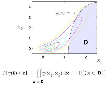
Fig. 40 Graphical depiction of calculation of cumulative distribution function in the original uncertain variable space.

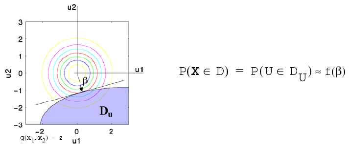
Fig. 41 Graphical depiction of integration for the calculation of cumulative distribution function in the transformed uncertain variable space.

Local Reliability Methods

The main section on Local Reliability Methods provides the algorithmic details for the local reliability methods, including the Mean Value method and the family of most probable point (MPP) search methods.

Method mapping

Given settings for limit state approximation, approximation order, integration approach, and other details presented to this point, it is evident that the number of algorithmic combinations is high. Table 8 provides a succinct mapping for some of these combinations to common method names from the reliability literature, where bold font indicates the most well-known combinations and regular font indicates other supported combinations.

Table 8 Mapping from Dakota options to standard reliability methods.
	Order of approximation and integration
MPP search	First order	Second order
none	MVFOSM	MVSOSM
x_taylor_mean	AMV	AMV\(^2\)
u_taylor_mean	u-space AMV	u-space AMV\(^2\)
x_taylor_mpp	AMV+	AMV\(^2\)+
u_taylor_mpp	u-space AMV+	u-space AMV\(^2\)+
x_two_point	TANA
u_two_point	u-space TANA
no_approx	FORM	SORM

Within the Dakota specification (refer to local_reliability), the MPP search and integration order selections are explicit in the method specification, but the order of the approximation is inferred from the associated response specification (as is done with local taylor series approximations described in Taylor Series). Thus, reliability methods do not have to be synchronized in approximation and integration order as shown in the table; however, it is often desirable to do so.

Global Reliability Methods

Global reliability methods are designed to handle nonsmooth and multimodal failure surfaces, by creating global approximations based on Gaussian process models. They accurately resolve a particular contour of a response function and then estimate probabilities using multimodal adaptive importance sampling.

The global reliability method in Dakota is called Efficient Global Reliability Analysis (EGRA) [BES+08]. The name is due to its roots in efficient global optimization (EGO) [HANZ06, JSW98]. The main idea in EGO-type optimization methods is that a global approximation is made of the underlying function. This approximation, which is a Gaussian process model, is used to guide the search by finding points which maximize the expected improvement function (EIF). The EIF is used to select the location at which a new training point should be added to the Gaussian process model by maximizing the amount of improvement in the objective function that can be expected by adding that point. A point could be expected to produce an improvement in the objective function if its predicted value is better than the current best solution, or if the uncertainty in its prediction is such that the probability of it producing a better solution is high. Because the uncertainty is higher in regions of the design space with fewer observations, this provides a balance between exploiting areas of the design space that predict good solutions, and exploring areas where more information is needed.

The general procedure of these EGO-type methods is:

Build an initial Gaussian process model of the objective function.
Find the point that maximizes the EIF. If the EIF value at this point is sufficiently small, stop.
Evaluate the objective function at the point where the EIF is maximized. Update the Gaussian process model using this new point. Go to Step 2.

Gaussian process (GP) models are used because they provide not just a predicted value at an unsampled point, but also an estimate of the prediction variance. This variance gives an indication of the uncertainty in the GP model, which results from the construction of the covariance function. This function is based on the idea that when input points are near one another, the correlation between their corresponding outputs will be high. As a result, the uncertainty associated with the model’s predictions will be small for input points which are near the points used to train the model, and will increase as one moves further from the training points.

The expected improvement function is used in EGO algorithms to select the location at which a new training point should be added. The EIF is defined as the expectation that any point in the search space will provide a better solution than the current best solution based on the expected values and variances predicted by the GP model. It is important to understand how the use of this EIF leads to optimal solutions. The EIF indicates how much the objective function value at a new potential location is expected to be less than the predicted value at the current best solution. Because the GP model provides a Gaussian distribution at each predicted point, expectations can be calculated. Points with good expected values and even a small variance will have a significant expectation of producing a better solution (exploitation), but so will points that have relatively poor expected values and greater variance (exploration).

The application of EGO to reliability analysis, however, is made more complicated due to the inclusion of equality constraints. In forward reliability analysis, the response function appears as a constraint rather than the objective. That is, we want to satisfy the constraint that the response equals a threshold value and is on the limit state: \(G({\bf u})\!=\!\bar{z}\). Therefore, the EIF function was modified to focus on feasibility, and instead of using an expected improvement function, we use an expected feasibility function (EFF) [BES+08]. The EFF provides an indication of how well the response is expected to satisfy the equality constraint. Points where the expected value is close to the threshold (\(\mu_G\!\approx\!\bar{z}\)) and points with a large uncertainty in the prediction will have large expected feasibility values.

The general outline of the EGRA algorithm is as follows: LHS sampling is used to generate a small number of samples from the true response function. Then, an initial Gaussian process model is constructed. Based on the EFF, the point with maximum EFF is found using the global optimizer DIRECT. The true response function is then evaluated at this new point, and this point is added to the sample set and the process of building a new GP model and maximizing the EFF is repeated until the maximum EFF is small. At this stage, the GP model is accurate in the vicinity of the limit state. The GP model is then used to calculate the probability of failure using multimodal importance sampling, which is explained below.

One method to calculate the probability of failure is to directly perform the probability integration numerically by sampling the response function. Sampling methods can be prohibitively expensive because they generally require a large number of response function evaluations. Importance sampling methods reduce this expense by focusing the samples in the important regions of the uncertain space. They do this by centering the sampling density function at the MPP rather than at the mean. This ensures the samples will lie the region of interest, thus increasing the efficiency of the sampling method. Adaptive importance sampling (AIS) further improves the efficiency by adaptively updating the sampling density function. Multimodal adaptive importance sampling [DM98] is a variation of AIS that allows for the use of multiple sampling densities making it better suited for cases where multiple sections of the limit state are highly probable.

Note that importance sampling methods require that the location of at least one MPP be known because it is used to center the initial sampling density. However, current gradient-based, local search methods used in MPP search may fail to converge or may converge to poor solutions for highly nonlinear problems, possibly making these methods inapplicable. The EGRA algorithm described above does not depend on the availability of accurate gradient information, making convergence more reliable for nonsmooth response functions. Moreover, EGRA has the ability to locate multiple failure points, which can provide multiple starting points and thus a good multimodal sampling density for the initial steps of multimodal AIS. The probability assessment using multimodal AIS thus incorporates probability of failure at multiple points.

Uncertainty Quantification Examples using Reliability Analysis

In summary, the user can choose to perform either forward (RIA) or inverse (PMA) mappings when performing a reliability analysis. With either approach, there are a variety of methods from which to choose in terms of limit state approximations (MVFOSM, MVSOSM, x-/u-space AMV, x-/u-space AMV\(^2\), x-/u-space AMV+, x-/u-space AMV\(^2\)+, x-/u-space TANA, and FORM/SORM), probability integrations (first-order or second-order), limit state Hessian selection (analytic, finite difference, BFGS, or SR1), and MPP optimization algorithm (SQP or NIP) selections.

All reliability methods output approximate values of the CDF/CCDF response-probability-reliability levels for prescribed response levels (RIA) or prescribed probability or reliability levels (PMA). In addition, mean value methods output estimates of the response means and standard deviations as well as importance factors that attribute variance among the set of uncertain variables (provided a nonzero response variance estimate).

Mean-value Reliability with Textbook

Listing 32 shows the Dakota input file for an example problem that demonstrates the simplest reliability method, called the mean value method (also referred to as the Mean Value First Order Second Moment method). It is specified with method keyword local_reliability. This method calculates the mean and variance of the response function based on information about the mean and variance of the inputs and gradient information at the mean of the inputs. The mean value method is extremely cheap computationally (only five runs were required for the textbook function), but can be quite inaccurate, especially for nonlinear problems and/or problems with uncertain inputs that are significantly non-normal. More detail on the mean value method can be found in the main Local Reliability Methods section, and more detail on reliability methods in general (including the more advanced methods) is found in Reliability Methods.

Example output from the mean value method is displayed in Listing 33. Note that since the mean of both inputs is 1, the mean value of the output for response 1 is zero. However, the mean values of the constraints are both 0.5. The mean value results indicate that variable x1 is more important in constraint 1 while x2 is more important in constraint 2, which is the case based on Textbook. The importance factors are not available for the first response as the standard deviation is zero.

Listing 32 Mean Value Reliability Method: the Dakota input file – see dakota/share/dakota/examples/users/textbook_uq_meanvalue.in

# Dakota Input File: textbook_uq_meanvalue.in

environment

method
  local_reliability

interface
  analysis_drivers = 'text_book'
    fork asynchronous

variables
  lognormal_uncertain = 2
    means                 =  1.      1.
    std_deviations        =  0.5     0.5
    descriptors           =  'TF1ln' 'TF2ln'

responses
  response_functions = 3
  numerical_gradients
    method_source dakota
    interval_type central
    fd_gradient_step_size = 1.e-4
  no_hessians

Listing 33 Results of the Mean Value Method on the Textbook Function

MV Statistics for response_fn_1:
  Approximate Mean Response                  =  0.0000000000e+00
  Approximate Standard Deviation of Response =  0.0000000000e+00
  Importance Factors not available.
MV Statistics for response_fn_2:
  Approximate Mean Response                  =  5.0000000000e-01
  Approximate Standard Deviation of Response =  1.0307764064e+00
  Importance Factor for TF1ln                =  9.4117647059e-01
  Importance Factor for TF2ln                =  5.8823529412e-02
MV Statistics for response_fn_3:
  Approximate Mean Response                  =  5.0000000000e-01
  Approximate Standard Deviation of Response =  1.0307764064e+00
  Importance Factor for TF1ln                =  5.8823529412e-02
  Importance Factor for TF2ln                =  9.4117647059e-01

FORM Reliability with Lognormal Ratio

This example quantifies the uncertainty in the “log ratio” response function:

\[g(x_1,x_2) = \frac{x_1}{x_2}\]

by computing approximate response statistics using reliability analysis to determine the response cumulative distribution function:

\[P[g(x_1,x_2) < \bar{z}]\]

where \(X_1\) and \(X_2\) are identically distributed lognormal random variables with means of 1, standard deviations of 0.5, and correlation coefficient of 0.3.

A Dakota input file showing RIA using FORM (option 7 in limit state approximations combined with first-order integration) is listed in Listing 34. The user first specifies the local_reliability method, followed by the MPP search approach and integration order. In this example, we specify mpp_search no_approx and utilize the default first-order integration to select FORM. Finally, the user specifies response levels or probability/reliability levels to determine if the problem will be solved using an RIA approach or a PMA approach. In the example of Listing 34, we use RIA by specifying a range of response_levels for the problem. The resulting output for this input is shown in Listing 35, with probability and reliability levels listed for each response level. Fig. 42 shows that FORM compares favorably to an exact analytic solution for this problem. Also note that FORM does have some error in the calculation of CDF values for this problem, but it is a very small error (on the order of e-11), much smaller than the error obtained when using a Mean Value method, which will be discussed next.

Listing 34 Dakota input file for Reliability UQ example using FORM – see dakota/share/dakota/examples/users/logratio_uq_reliability.in

# Dakota Input File: logratio_uq_reliability.in

environment

method
  local_reliability
    mpp_search no_approx
    response_levels = .4 .5 .55 .6 .65 .7
     .75 .8 .85 .9 1. 1.05 1.15 1.2 1.25 1.3
     1.35 1.4 1.5 1.55 1.6 1.65 1.7 1.75

variables
  lognormal_uncertain = 2
    means             =  1.  1
    std_deviations    =  0.5 0.5
    initial_point     =  0.6 1.4
    descriptors       =  'TF1ln'   'TF2ln'
  uncertain_correlation_matrix =  1   0.3
            0.3 1

interface
  analysis_drivers = 'log_ratio'
    direct
#  fork asynch

responses
  response_functions = 1
  numerical_gradients
    method_source dakota
    interval_type central
    fd_step_size = 1.e-4
  no_hessians

Listing 35 Output from Reliability UQ example using FORM.

Cumulative Distribution Function (CDF) for response_fn_1:
     Response Level  Probability Level  Reliability Index
     --------------  -----------------  -----------------
0000000000e-01   4.7624085962e-02   1.6683404020e+00
0000000000e-01   1.0346525475e-01   1.2620507942e+00
5000000000e-01   1.3818404972e-01   1.0885143628e+00
0000000000e-01   1.7616275822e-01   9.3008801339e-01
5000000000e-01   2.1641741368e-01   7.8434989943e-01
0000000000e-01   2.5803428381e-01   6.4941748143e-01
5000000000e-01   3.0020938124e-01   5.2379840558e-01
0000000000e-01   3.4226491013e-01   4.0628960782e-01
5000000000e-01   3.8365052982e-01   2.9590705956e-01
0000000000e-01   4.2393548232e-01   1.9183562480e-01
0000000000e+00   5.0000000000e-01   6.8682233460e-12
0500000000e+00   5.3539344228e-01  -8.8834907167e-02
1500000000e+00   6.0043460094e-01  -2.5447217462e-01
2000000000e+00   6.3004131827e-01  -3.3196278078e-01
2500000000e+00   6.5773508987e-01  -4.0628960782e-01
3000000000e+00   6.8356844630e-01  -4.7770089473e-01
3500000000e+00   7.0761025532e-01  -5.4641676380e-01
4000000000e+00   7.2994058691e-01  -6.1263331274e-01
5000000000e+00   7.6981945355e-01  -7.3825238860e-01
5500000000e+00   7.8755158269e-01  -7.9795460350e-01
6000000000e+00   8.0393505584e-01  -8.5576118635e-01
6500000000e+00   8.1906005158e-01  -9.1178881995e-01
7000000000e+00   8.3301386860e-01  -9.6614373461e-01
7500000000e+00   8.4588021938e-01  -1.0189229206e+00

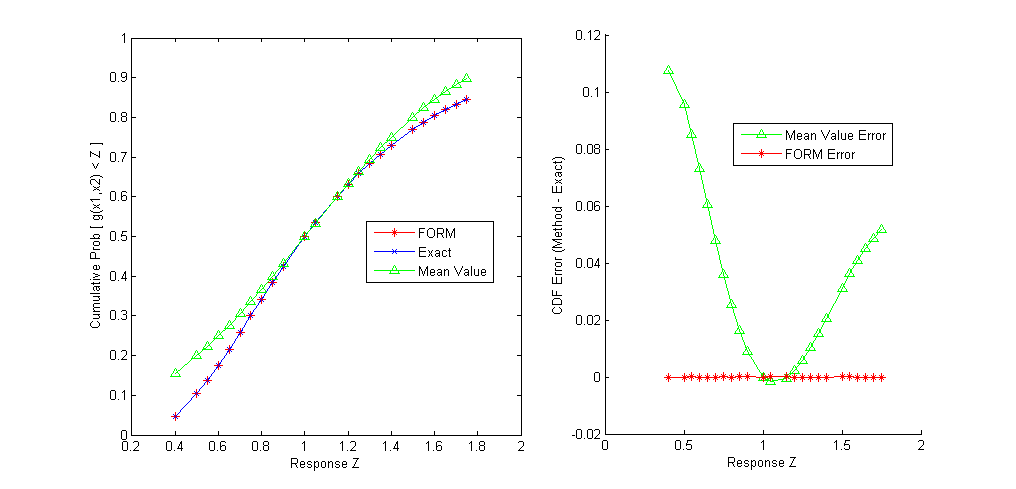
Comparison of the cumulative distribution function (CDF) computed by FORM, the Mean Value method, and the exact CDF for :math:`g(x_1,x_2)=\frac{x_1}{x_2}` — Fig. 42 Comparison of the cumulative distribution function (CDF) computed by FORM, the Mean Value method, and the exact CDF for \(g(x_1,x_2)=\frac{x_1}{x_2}\)

If the user specifies local_reliability as a method with no additional specification on how to do the MPP search (for example, by commenting out mpp_search no_approx in Listing 34), then no MPP search is done: the Mean Value method is used. The mean value results are shown in Listing 36 and consist of approximate mean and standard deviation of the response, the importance factors for each uncertain variable, and approximate probability/reliability levels for the prescribed response levels that have been inferred from the approximate mean and standard deviation (see the Mean Value section of the main Reliability Methods page). It is evident that the statistics are considerably different from the fully converged FORM results; however, these rough approximations are also much less expensive to calculate. The importance factors are a measure of the sensitivity of the response function(s) to the uncertain input variables. A comparison of the mean value results with the FORM results is shown in Fig. 42. The mean value results are not accurate near the tail values of the CDF, and can differ from the exact solution by as much as 0.11 in CDF estimates. A comprehensive comparison of various reliability methods applied to the logratio problem is provided in [EB06].

Listing 36 Output from Reliability UQ example using mean value.

MV Statistics for response_fn_1:
  Approximate Mean Response                  =  1.0000000000e+00
  Approximate Standard Deviation of Response =  5.9160798127e-01
  Importance Factor for TF1ln                =  7.1428570714e-01
  Importance Factor for TF2ln                =  7.1428572143e-01
  Importance Factor for TF1ln     TF2ln      = -4.2857142857e-01
Cumulative Distribution Function (CDF) for response_fn_1:
     Response Level  Probability Level  Reliability Index  General Rel Index
     --------------  -----------------  -----------------  -----------------
0000000000e-01   1.5524721837e-01   1.0141851006e+00   1.0141851006e+00
0000000000e-01   1.9901236093e-01   8.4515425050e-01   8.4515425050e-01
5000000000e-01   2.2343641149e-01   7.6063882545e-01   7.6063882545e-01
0000000000e-01   2.4948115037e-01   6.7612340040e-01   6.7612340040e-01
5000000000e-01   2.7705656603e-01   5.9160797535e-01   5.9160797535e-01
0000000000e-01   3.0604494093e-01   5.0709255030e-01   5.0709255030e-01
5000000000e-01   3.3630190949e-01   4.2257712525e-01   4.2257712525e-01
0000000000e-01   3.6765834596e-01   3.3806170020e-01   3.3806170020e-01
5000000000e-01   3.9992305332e-01   2.5354627515e-01   2.5354627515e-01
0000000000e-01   4.3288618783e-01   1.6903085010e-01   1.6903085010e-01
0000000000e+00   5.0000000000e-01   0.0000000000e+00   0.0000000000e+00
0500000000e+00   5.3367668035e-01  -8.4515425050e-02  -8.4515425050e-02
1500000000e+00   6.0007694668e-01  -2.5354627515e-01  -2.5354627515e-01
2000000000e+00   6.3234165404e-01  -3.3806170020e-01  -3.3806170020e-01
2500000000e+00   6.6369809051e-01  -4.2257712525e-01  -4.2257712525e-01
3000000000e+00   6.9395505907e-01  -5.0709255030e-01  -5.0709255030e-01
3500000000e+00   7.2294343397e-01  -5.9160797535e-01  -5.9160797535e-01
4000000000e+00   7.5051884963e-01  -6.7612340040e-01  -6.7612340040e-01
5000000000e+00   8.0098763907e-01  -8.4515425050e-01  -8.4515425050e-01
5500000000e+00   8.2372893005e-01  -9.2966967555e-01  -9.2966967555e-01
6000000000e+00   8.4475278163e-01  -1.0141851006e+00  -1.0141851006e+00
6500000000e+00   8.6405064339e-01  -1.0987005257e+00  -1.0987005257e+00
7000000000e+00   8.8163821351e-01  -1.1832159507e+00  -1.1832159507e+00
7500000000e+00   8.9755305196e-01  -1.2677313758e+00  -1.2677313758e+00

Additional reliability analysis and design results are provided in Sections Log Ratio through Steel Column.

Stochastic Expansion Methods

The development of these techniques mirrors that of deterministic finite element analysis through the utilization of the concepts of projection, orthogonality, and weak convergence. The polynomial chaos expansion is based on a multidimensional orthogonal polynomial approximation and the stochastic collocation approach is based on a multidimensional interpolation polynomial approximation, both formed in terms of standardized random variables. A distinguishing feature of these two methodologies is that the final solution is expressed as a functional mapping, and not merely as a set of statistics as is the case for many other methodologies (sampling, reliability, et al.). This makes these techniques particularly attractive for use in multi-physics applications which link different analysis packages. The first stochastic expansion method is the polynomial chaos expansion (PCE) [GRH99, GS91]. For smooth functions (i.e., analytic, infinitely-differentiable) in \(L^2\) (i.e., possessing finite variance), exponential convergence rates can be obtained under order refinement for integrated statistical quantities of interest such as mean, variance, and probability. Dakota implements the generalized PCE approach using the Wiener-Askey scheme [XK02], in which Hermite, Legendre, Laguerre, Jacobi, and generalized Laguerre orthogonal polynomials are used for modeling the effect of continuous random variables described by normal, uniform, exponential, beta, and gamma probability distributions, respectively 1. These orthogonal polynomial selections are optimal for these distribution types since the inner product weighting function corresponds 2 to the probability density functions for these continuous distributions. Orthogonal polynomials can be computed for any positive weight function, so these five classical orthogonal polynomials may be augmented with numerically-generated polynomials for other probability distributions (e.g., for lognormal, extreme value, and histogram distributions). When independent standard random variables are used (or computed through transformation), the variable expansions are uncoupled, allowing the polynomial orthogonality properties to be applied on a per-dimension basis. This allows one to mix and match the polynomial basis used for each variable without interference with the spectral projection scheme for the response.

In non-intrusive PCE, simulations are used as black boxes and the calculation of chaos expansion coefficients for response metrics of interest is based on a set of simulation response evaluations. To calculate these response PCE coefficients, two classes of approaches are available: spectral projection and regression. The spectral projection approach projects the response against each basis function using inner products and employs the polynomial orthogonality properties to extract each coefficient. Each inner product involves a multidimensional integral over the support range of the weighting function, which can be evaluated numerically using sampling, tensor-product quadrature, Smolyak sparse grid [Smo63], or cubature [Str71] approaches. The regression approach finds a set of PCE coefficients which best match a set of response values obtained from either a design of computer experiments (“point collocation” [Wal03]) or from a randomly selected subset of tensor Gauss points (“probabilistic collocation” [Tat95]). Various methods can be used to solve the resulting linear system, including least squares methods for over-determined systems and compressed sensing methods for under-determined systems. Details of these methods are documented in Linear regression and the necessary specifications needed to activate these techniques are provided in the documentation for the polynomial_chaos keyword.

Stochastic collocation (SC) is another stochastic expansion technique for UQ that is closely related to PCE. As for PCE, exponential convergence rates can be obtained under order refinement for integrated statistical quantities of interest, provided that the response functions are smooth with finite variance. The primary distinction is that, whereas PCE estimates coefficients for known multivariate orthogonal polynomial basis functions, SC forms multivariate interpolation polynomial basis functions for known coefficients. The interpolation polynomials may be either local or global and either value-based or gradient-enhanced (four combinations: Lagrange interpolation, Hermite interpolation, piecewise linear spline, and piecewise cubic spline), and may be used within nodal or hierarchical interpolation formulations. Interpolation is performed on structured grids such as tensor-product or sparse grids. Starting from a tensor-product multidimensional interpolation polynomial in the value-based case (Lagrange or piecewise linear spline), we have the feature that the \(i^{th}\) interpolation polynomial has a value of 1 at collocation point \(i\) and a value of 0 for all other collocation points, leading to the use of expansion coefficients that are just the response values at each of the collocation points. In the gradient-enhanced case (Hermite or piecewise cubic spline), SC includes both “type 1” and “type 2” interpolation polynomials, where the former interpolate the values while producing zero gradients and the latter interpolate the gradients while producing zero values. Sparse interpolants are weighted sums of these tensor interpolants;

however, they are only interpolatory for sparse grids based on fully nested rules and will exhibit some interpolation error at the collocation points for sparse grids based on non-nested rules. A key to maximizing performance with SC is performing collocation using the Gauss points and weights from the same optimal orthogonal polynomials used in PCE. For use of standard Gauss integration rules (not nested variants such as Gauss-Patterson or Genz-Keister) within tensor-product quadrature, tensor PCE expansions and tensor SC interpolants are equivalent in that identical polynomial approximations are generated [CGI10]. Moreover, this equivalence can be extended to sparse grids based on standard Gauss rules, provided that a sparse PCE is formed based on a weighted sum of tensor expansions [CEP12].

Note

Stochastic Expansion Methods provides full algorithmic details for the PCE and SC methods.

A recent addition is functional tensor train (FTT) expansions which leverage concepts from data/image compression using products of dimensional basis “cores.” When the response admits a “low rank” representation, this means that the size of the cores required for an accurate recovery is not large and a compressed format for the expansion can be achieved based on a tensor train composition. In Dakota, the basis functions used within the core for each random dimension are univariate orthogonal polynomials, similar to PCE. Solution for the expansion coefficients is based on regression and employs a numerical solution of a regularized nonlinear least squares problem. Both the rank and polynomial order per dimension are resolution controls for the method, and cross-validation procedures are provided to automate the selection of the best settings for a given response data set. Additional FTT theory will be provided in future releases as this capability is promoted to a default part of the Dakota software configuration.

Finally, advanced multilevel and multifidelity approaches are provided for PCE, SC, and FT (refer to multilevel_polynomial_chaos, multifidelity_polynomial_chaos, multilevel_function_train, multifidelity_function_train and multifidelity_stoch_collocation). These approaches decompose the input-output mapping and form multiple expansions in order to reduce reliance on the most expensive computational models by integrating information from low cost modeling alternatives.

Uncertainty Quantification Examples using Stochastic Expansions

Polynomial Chaos Expansion for Rosenbrock

A typical Dakota input file for performing an uncertainty quantification using PCE is shown in Listing 37. In this example, we compute CDF probabilities for six response levels of Rosenbrock’s function. Since Rosenbrock is a fourth order polynomial and we employ a fourth-order expansion using an optimal basis (Legendre for uniform random variables), we can readily obtain a polynomial expansion which exactly matches the Rosenbrock function. In this example, we select Gaussian quadratures using an anisotropic approach (fifth-order quadrature in \(x_1\) and third-order quadrature in \(x_2\)), resulting in a total of 15 function evaluations to compute the PCE coefficients.

Listing 37 Dakota input file for performing UQ using polynomial chaos expansions – see dakota/share/dakota/examples/users/rosen_uq_pce.in

# Dakota Input File: rosen_uq_pce.in

environment

method
  polynomial_chaos
    quadrature_order = 5
    dimension_preference = 5 3
    samples_on_emulator = 10000
    seed = 12347
    response_levels = .1 1. 50. 100. 500. 1000.
    variance_based_decomp #interaction_order = 1

variables
  uniform_uncertain = 2
    lower_bounds      = -2.  -2.
    upper_bounds      =  2.   2.
    descriptors       = 'x1' 'x2'

interface
  analysis_drivers = 'rosenbrock'
    direct

responses
  response_functions = 1
  no_gradients
  no_hessians

The tensor product quadature points upon which the expansion is calculated are shown in Fig. 43. The tensor product generates all combinations of values from each individual dimension: it is an all-way pairing of points.

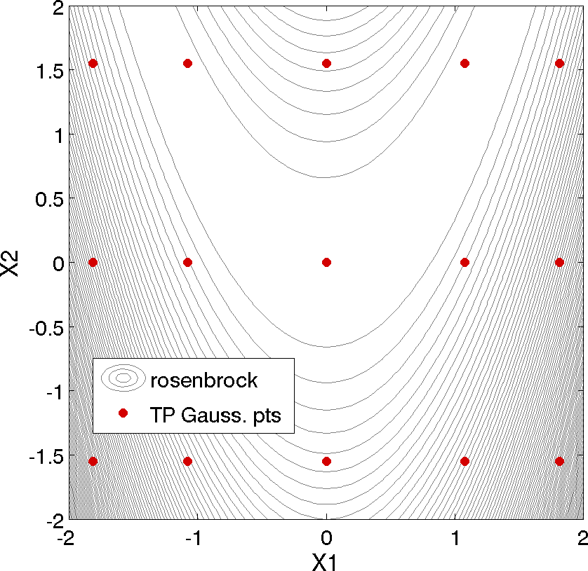
Fig. 43 Rosenbrock polynomial chaos example: tensor product quadrature points.

Once the expansion coefficients have been calculated, some statistics are available analytically and others must be evaluated numerically. For the numerical portion, the input file specifies the use of 10000 samples, which will be evaluated on the expansion to compute the CDF probabilities. In Listing 38, excerpts from the results summary are presented, where we first see a summary of the PCE coefficients which exactly reproduce Rosenbrock for a Legendre polynomial basis. The analytic statistics for mean, standard deviation, and COV are then presented. For example, the mean is 455.66 and the standard deviation is 606.56. The moments are followed by global sensitivity indices (Sobol’ indices).This example shows that variable x1 has the largest main effect (0.497) as compared with variable x2 (0.296) or the interaction between x1 and x2 (0.206). After the global sensitivity indices, the local sensitivities are presented, evaluated at the mean values. Finally, we see the numerical results for the CDF probabilities based on 10000 samples performed on the expansion. For example, the probability that the Rosenbrock function is less than 100 over these two uncertain variables is 0.342. Note that this is a very similar estimate to what was obtained using 200 Monte Carlo samples, with fewer true function evaluations.

Listing 38 Excerpt of UQ output for polynomial chaos example.

Polynomial Chaos coefficients for response_fn_1:
        coefficient   u1   u2
        ----------- ---- ----
   4.5566666667e+02   P0   P0
  -4.0000000000e+00   P1   P0
   9.1695238095e+02   P2   P0
  -9.9475983006e-14   P3   P0
   3.6571428571e+02   P4   P0
  -5.3333333333e+02   P0   P1
  -3.9968028887e-14   P1   P1
  -1.0666666667e+03   P2   P1
  -3.3573144265e-13   P3   P1
   1.2829737273e-12   P4   P1
   2.6666666667e+02   P0   P2
   2.2648549702e-13   P1   P2
   4.8849813084e-13   P2   P2
   2.8754776338e-13   P3   P2
  -2.8477220582e-13   P4   P2
-------------------------------------------------------------------
Statistics derived analytically from polynomial expansion:

Moment-based statistics for each response function:
                            Mean           Std Dev          Skewness          Kurtosis
response_fn_1
  expansion:    4.5566666667e+02  6.0656024184e+02
  numerical:    4.5566666667e+02  6.0656024184e+02  1.9633285271e+00  3.3633861456e+00

Covariance among response functions:
[[  3.6791532698e+05 ]]

Local sensitivities for each response function evaluated at uncertain variable means:
response_fn_1:
 [ -2.0000000000e+00  2.4055757386e-13 ]

Global sensitivity indices for each response function:
response_fn_1 Sobol indices:
                                  Main             Total
                      4.9746891383e-01  7.0363551328e-01 x1
                      2.9636448672e-01  5.0253108617e-01 x2
                           Interaction
                      2.0616659946e-01 x1 x2

Statistics based on 10000 samples performed on polynomial expansion:

Probability Density Function (PDF) histograms for each response function:
PDF for response_fn_1:
          Bin Lower          Bin Upper      Density Value
          ---------          ---------      -------------
   6.8311107124e-03   1.0000000000e-01   2.0393073423e-02
   1.0000000000e-01   1.0000000000e+00   1.3000000000e-02
   1.0000000000e+00   5.0000000000e+01   4.7000000000e-03
   5.0000000000e+01   1.0000000000e+02   1.9680000000e-03
   1.0000000000e+02   5.0000000000e+02   9.2150000000e-04
   5.0000000000e+02   1.0000000000e+03   2.8300000000e-04
   1.0000000000e+03   3.5755437782e+03   5.7308286215e-05

Level mappings for each response function:
Cumulative Distribution Function (CDF) for response_fn_1:
     Response Level  Probability Level  Reliability Index  General Rel Index
     --------------  -----------------  -----------------  -----------------
   1.0000000000e-01   1.9000000000e-03
   1.0000000000e+00   1.3600000000e-02
   5.0000000000e+01   2.4390000000e-01
   1.0000000000e+02   3.4230000000e-01
   5.0000000000e+02   7.1090000000e-01
   1.0000000000e+03   8.5240000000e-01
-------------------------------------------------------------------

Uncertainty Quantification Example using Stochastic Collocation

Compared to the previous PCE example, this section presents a more sophisticated example, where we use stochastic collocation built on an anisotropic sparse grid defined from numerically-generated orthogonal polynomials. The uncertain variables are lognormal in this example and the orthogonal polynomials are generated from Gauss-Wigert recursion coefficients [Sim78] in combination with the Golub-Welsch procedure [GW69]. The input file is shown in Listing 39. Note that the dimension preference of \((2,1)\) is inverted to define a \(\gamma\) weighting vector of \((0.5,1)\) (and \(\underline{\gamma}\) of \(0.5\)) for use in the anisotropic Smolyak index set constraint (see Smolyak sparse grids). In this example, we compute CDF probabilities for six response levels of Rosenbrock’s function. This example requires 19 function evaluations to calculate the interpolating polynomials in stochastic collocation and the resulting expansion exactly reproduces Rosenbrock’s function. The placement of the points generated by the sparse grid is shown in Fig. 44.

Listing 39 Dakota input file for performing UQ using stochastic collocation – see dakota/share/dakota/examples/users/rosen_uq_sc.in

# Dakota Input File: rosen_uq_sc.in

environment

method
  stoch_collocation
    sparse_grid_level = 3
    dimension_preference = 2 1
    samples_on_emulator = 10000 seed = 12347
    response_levels = .1 1. 50. 100. 500. 1000.
    variance_based_decomp #interaction_order = 1
  output silent

variables
  lognormal_uncertain = 2
    means             =  1.   1.
    std_deviations    =  0.5  0.5
    descriptors       = 'x1' 'x2'

interface
  analysis_drivers = 'rosenbrock'
    direct

responses
  response_functions = 1
  no_gradients
  no_hessians

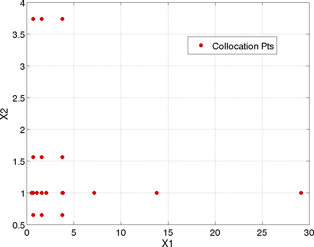
Fig. 44 Rosenbrock stochastic collocation example: sparse grid points.

Once the expansion coefficients have been calculated, some statistics are available analytically and others must be evaluated numerically. For the numerical portion, the input file specifies the use of 10000 samples, which will be evaluated on the expansion to compute the CDF probabilities. In Listing 40, excerpts from the results summary are presented. We first see the moment statistics for mean, standard deviation, skewness, and kurtosis computed by numerical integration (see Analytic moments), where the numerical row corresponds to integration using the original response values and the expansion row corresponds to integration using values from the interpolant. The response covariance (collapsing to a single variance value for one response function) and global sensitivity indices (Sobol’ indices) are presented next. This example shows that variable x1 has the largest main effect (0.99) as compared with variable x2 (0.0007) or the interaction between x1 and x2 (0.005).

Finally, we see the numerical results for the CDF probabilities based on 10000 samples performed on the expansion. For example, the probability that the Rosenbrock function is less than 100 is 0.7233. Note that these results are significantly different than the ones presented in Polynomial Chaos Expansion for Rosenbrock because of the different assumptions about the inputs: uniform[-2,2] versus lognormals with means of 1.0 and standard deviations of 0.5.

Listing 40 Excerpt of UQ output for stochastic collocation example.

Statistics derived analytically from polynomial expansion:

Moment-based statistics for each response function:
                            Mean           Std Dev          Skewness          Kurtosis
response_fn_1
  expansion:    2.5671972656e+02  2.0484189184e+03  2.7419241630e+02  1.9594567379e+06
  numerical:    2.5671972656e+02  2.0484189184e+03  2.7419241630e+02  1.9594567379e+06

Covariance among response functions:
[[  4.1960200651e+06 ]]

Global sensitivity indices for each response function:
response_fn_1 Sobol indices:
                                  Main             Total
                      9.9391978710e-01  9.9928724777e-01 x1
                      7.1275222945e-04  6.0802128961e-03 x2
                           Interaction
                      5.3674606667e-03 x1 x2

Statistics based on 10000 samples performed on polynomial expansion:

Level mappings for each response function:
Cumulative Distribution Function (CDF) for response_fn_1:
     Response Level  Probability Level  Reliability Index  General Rel Index
     --------------  -----------------  -----------------  -----------------
   1.0000000000e-01   1.8100000000e-02
   1.0000000000e+00   8.7800000000e-02
   5.0000000000e+01   5.8410000000e-01
   1.0000000000e+02   7.2330000000e-01
   5.0000000000e+02   9.2010000000e-01
   1.0000000000e+03   9.5660000000e-01

Importance Sampling Methods

Importance sampling is a method that allows one to estimate statistical quantities such as failure probabilities (e.g. the probability that a response quantity will exceed a threshold or fall below a threshold value) in a way that is more efficient than Monte Carlo sampling. The core idea in importance sampling is that one generates samples that preferentially samples important regions in the space (e.g. in or near the failure region or user-defined region of interest), and then appropriately weights the samples to obtain an unbiased estimate of the failure probability [Sri02]. In importance sampling, the samples are generated from a density which is called the importance density: it is not the original probability density of the input distributions. The importance density should be centered near the failure region of interest. For black-box simulations such as those commonly interfaced with Dakota, it is difficult to specify the importance density a priori: the user often does not know where the failure region lies, especially in a high-dimensional space. [SW10]

More formally, we define the objective of importance sampling as calculating the probability, \(P\), that the output will exceed a threshold level. This is a failure probability, where the failure probability is defined as some scalar function, \(y\left(\textbf{X}\right)\), exceeding a threshold, \(T\), where the inputs, \(\textbf{X}\), are randomly distributed with density, \(\rho\left(\textbf{X}\right)\). When evaluating \(y\left(\textbf{X}\right)\) is sufficiently expensive or \(P\) is sufficiently small, Monte Carlo (MC) sampling methods to estimate \(P\) will be infeasible due to the large number of function evaluations required for a specified accuracy.

The probability of failure can be thought of as the mean rate of occurrence of failure. The Monte Carlo (MC) estimate of \(P\) is therefore the sample mean of the indicator function, \(I\left(\textbf{X}\right)\),

(26)\[P_{MC}=\frac{1}{N}\sum_{i=1}^{N}I\left(\mathbf{X_i}\right)\ \ \textbf{X}\sim \rho\left(\textbf{X}\right),\]

where \(N\) samples, \(\mathbf{X_i}\), are drawn from \(\rho\left(\textbf{X}\right)\), and the indicator function \(I\left(\textbf{X}\right)\) is 1 if failure occurs and zero otherwise.

Importance sampling draws samples from the importance density \(\rho'\left(\textbf{X}\right)\) and scales the sample mean by the importance density:

(27)\[P_{IS}=\frac{1}{N}\sum_{i=1}^N \left(I\left(\mathbf{X_i}\right)\frac{\rho\left(\mathbf{X_i}\right)}{\rho'\left(\mathbf{X_i}\right)}\right)\ \ \textbf{X}\sim\rho'\left(\textbf{X}\right).\]

This reduces the asymptotic error variance from:

\[\sigma_{err_{MC}}^2=\frac{{\rm E}\left[\left(I\left(\textbf{X}\right)-P\right)^2\right]}{N}\]

to

(28)\[\sigma_{err_{IS}}^2=\frac{{\rm E}\left[\left(I\left(\textbf{X}\right)\frac{\rho\left(\textbf{X}\right)}{\rho'\left(\textbf{X}\right)} -P\right)^2\right]}{N}.\]

Inspection of Eq. (28) reveals \(\sigma_{err_{IS}}^2=0\) if \(\rho'\left(\textbf{X}\right)\) equals the ideal importance density \(\rho^*\left(\textbf{X}\right)\),

\[\rho^*\left(\textbf{X}\right)=\frac{I\left(\textbf{X}\right)\rho\left(\textbf{X}\right)}{P}.\]

However, \(\rho^*\left(\textbf{X}\right)\) is unknown a priori because \(I\left(\textbf{X}\right)\) is only known where it has been evaluated. Therefore, the required \(P\) in the denominator is also unknown: this is what we are trying to estimate.

If importance sampling is to be effective, the practitioner must be able to choose a good \(\rho'\left(\textbf{X}\right)\) without already knowing \(I\left(\textbf{X}\right)\) everywhere. There is a danger: a poor choice for \(\rho'\left(\textbf{X}\right)\) can put most of the samples in unimportant regions and make \(\sigma_{err_{IS}}^2\) much greater than \(\sigma_{err_{MC}}^2\). In particular, importance sampling can be challenging for very low probability events in high-dimensional spaces where the output \(y\) is calculated by a simulation. In these cases, usually one does not know anything a priori about where the failure region exists in input space. We have developed two importance sampling approaches which do not rely on the user explicitly specifying an importance density.

Importance Sampling Method based on Reliability Approach

The first method is based on ideas in reliability modeling Local Reliability Methods. An initial Latin Hypercube sampling is performed to generate an initial set of samples. These initial samples are augmented with samples from an importance density as follows: The variables are transformed to standard normal space. In the transformed space, the importance density is a set of normal densities centered around points which are in the failure region. Note that this is similar in spirit to the reliability methods, in which importance sampling is centered around a Most Probable Point (MPP). In the case of the LHS samples, the importance sampling density will simply by a mixture of normal distributions centered around points in the failure region.

This method is specified by the keyword importance_sampling. The options for importance sampling are as follows: import centers a sampling density at one of the initial LHS samples identified in the failure region. It then generates the importance samples, weights them by their probability of occurence given the original density, and calculates the required probability (CDF or CCDF level). adapt_import is the same as import but is performed iteratively until the failure probability estimate converges. mm_adapt_import starts with all of the samples located in the failure region to build a multimodal sampling density. First, it uses a small number of samples around each of the initial samples in the failure region. Note that these samples are allocated to the different points based on their relative probabilities of occurrence: more probable points get more samples. This early part of the approach is done to search for “representative” points. Once these are located, the multimodal sampling density is set and then the multi-modal adaptive method proceeds similarly to the adaptive method (sample until convergence).

Gaussian Process Adaptive Importance Sampling Method

The second importance sampling method in Dakota is the one we recommend, at least for problems that have a relatively small number of input variables (e.g. less than 10). This method, Gaussian Process Adaptive Importance Sampling, is outlined in the paper [DS14]. This method starts with an initial set of LHS samples and adds samples one at a time, with the goal of adaptively improving the estimate of the ideal importance density during the process. The approach uses a mixture of component densities. An iterative process is used to construct the sequence of improving component densities. At each iteration, a Gaussian process (GP) surrogate is used to help identify areas in the space where failure is likely to occur. The GPs are not used to directly calculate the failure probability; they are only used to approximate the importance density. Thus, the Gaussian process adaptive importance sampling algorithm overcomes limitations involving using a potentially inaccurate surrogate model directly in importance sampling calculations.

This method is specified with the keyword gpais. There are three main controls which govern the behavior of the algorithm. samples specifies the initial number of Latin Hypercube samples which are used to create the initial Gaussian process surrogate. emulator_samples specifies the number of samples taken on the latest Gaussian process model each iteration of the algorithm. These samples are used in the construction of the next importance sampling density. The default is 10,000 samples. The third control is max_iterations, which controls the number of iterations of the algorithm. Each iteration, one additional sample of the “true” simulation is taken. Thus, if samples were set at 100 and max_iterations were set to 200, there would be a total of 300 function evaluations of the simulator model taken.

Adaptive Sampling Methods

The goal in performing adaptive sampling is to construct a surrogate model that can be used as an accurate predictor to some expensive simulation, thus it is to one’s advantage to build a surrogate that minimizes the error over the entire domain of interest using as little data as possible from the expensive simulation. The adaptive part alludes to the fact that the surrogate will be refined by focusing samples of the expensive simulation on particular areas of interest rather than rely on random selection or standard space-filling techniques.

Adaptive sampling based on surrogates

At a high-level, the adaptive sampling pipeline is a four-step process:

Evaluate the expensive simulation (referred to as the true model) at initial sample points
Fit/refit a surrogate model
Create a candidate set and score based on information from surrogate
Select a candidate point to evaluate the true model and Repeat 2-4

In terms of the Dakota implementation, the adaptive sampling method currently uses Latin Hypercube sampling (LHS) to generate the initial points in Step 1 above. For Step 2, we use a Gaussian process model. The user can specify the scoring metric used to select the next point (or points) to evaluate and add to the set. We have investigated several scoring metrics with which to evaluate candidate points for Step 3. There are some classical ones such as distance (e.g. add a point which maximizes the minimum distance to all of the existing points). This distance metric tends to generate points that are space-filling. We have investigated several methods that involve interesting topological features of the space (e.g. points that are near saddle points). These are an area of active investigation but are not currently included in Dakota. The fitness metrics for scoring candidate points currently include:

Predicted Variance: First introduced in [Mac92] and later used in [SWGO00], this method uses the predicted variance of the Gaussian process surrogate as the score of a candidate point. Thus, the adaptively chosen points will be in areas of highest uncertainty according to the Gaussian process model.
Distance: A candidate’s score is the Euclidean distance in domain space between the candidate and its nearest neighbor in the set of points already evaluated on the true model. Therefore, the most undersampled area of the domain will always be selected. The adaptivity of this method could be brought to question as it would chose the exact same points regardless of the surrogate model used. However, it is useful to use to compare other adaptive metrics to one that relies purely on space-filling in an equivalent context.

Gradient: Similar to the above metric, a candidate’s nearest neighbor is determined as in the distance metric, only now the score is the absolute value of the difference in range space of the two points. The range space values used are predicted from the surrogate model. Though this method is called the gradient metric, it actually does not take into account how close the candidate and its neighbor are in domain space. This method attempts to evenly fill the range space of the surrogate.

Note that in our approach, a Latin Hypercube sample is generated (a new one, different from the initial sample) and the surrogate model is evaluated at this points. These are the “candidate points” that are then evaluated according to the fitness metric outlined above. The number of candidates used in practice should be high enough to fill most of the input domain: we recommend at least hundreds of points for a low- dimensional problem. All of the candidates (samples on the emulator) are given a score and then the highest-scoring candidate is selected to be evaluated on the true model.

The adaptive sampling method also can generate batches of points to add at a time. With batch or multi-point selection, the true model can be evaluated in parallel and thus increase throughput before refitting our surrogate model. This proposes a new challenge as the problem of choosing a single point and choosing multiple points off a surrogate are fundamentally different. Selecting the \(n\) best scoring candidates is more than likely to generate a set of points clustered in one area which will not be conducive to adapting the surrogate. We have implemented several strategies for batch selection of points:

Naive Selection: This strategy will select the \(n\) highest scoring candidates regardless of their position. This tends to group an entire round of points in the same area.
Distance Penalized Re-weighted Scoring: In this strategy, the highest scoring candidate is selected and then all remaining candidates are re-scored with a distance penalization factor added in to the score. Only points selected within a round are used for the distance penalization. The factor is the same as used in the distance penalization scoring metrics from [MWK+12]. First, compute all of the minimum distances from each remaining candidate to the selected candidates. Then, determine the median value of these distances. If the smallest distance, \(d\), between a point and the selected set is less than the computed median distance its score is unaltered, otherwise the score is multiplied by a value \(\rho\) determined by the following equation:

\[\rho = 1.5*d - 0.5*d^3\]
Topological Maxima of Scoring Function: In this strategy we look at the topology of the scoring function and select the \(n\) highest maxima in the topology. To determine local maxima, we construct the approximate Morse-Smale complex. If the number of local maxima is less than \(n\), we revert to the distance strategy above. As a further extension, one may want to filter low-persistence maxima, but to keep the framework general, we chose to omit this feature as defining a threshold for what deems a critical point as “low persistence” can vary drastically from problem to problem.
Constant Liar: We adapt the constant liar strategy presented in [GRC10] with the scoring metrics. The strategy first selects the highest scoring candidate, and then refits the surrogate using a “lie” value at the point selected and repeating until \(n\) points have been selected whereupon the lie values are removed from the surrogate and the selected points are evaluated on the true model and the surrogate is refit with these values.

The adaptive sampling method is specified by the method keyword adaptive_sampling. There are many controls, including the number of candidate samples to investigate each iteration (emulator_samples), the fitness metric used in scoring candidates (fitness_metric), and the number of iterations to perform the adaptive sampling (max_iterations). For batch selection of points, one specifies a batch_selection strategy and a batch_size. The details of the specification are provided in the Dakota reference manual.

Adaptive sampling based on dart throwing

pof_darts is a novel method for estimating the tail probability (Probability of Failure) based on random sphere-packing in the uncertain parameter space. Random points are sequentially sampled from the domain and consequently surrounded by protecting spheres, with the constraint that each new sphere center has to be outside all prior spheres [EMS+16]. The radius of each sphere is chosen such that the entire sphere lies either in the failure or the non-failure region. This radius depends of the function evaluation at the disk center, the failure threshold and an estimate of the function gradient at the disk center. After exhausting the sampling budget specified by build_samples, which is the number of spheres per failure threshold, the domain is decomposed into two regions. These regions correspond to failure and non-failure categories, each represented by the union of the spheres of each type. The volume of the union of failure spheres gives a lower bound on the required estimate of the probability of failure, while the volume of the union of the non-failure spheres subtracted from the volume of the domain gives an upper estimate. After all the spheres are constructed, we construct a surrogate model, specified via a model_pointer, and sample the surrogate model extensively to estimate the probability of failure for each threshold.

pof_darts handles multiple response functions and allows each to have multiple failure thresholds. For each failure threshold pof_darts will insert a number of spheres specified by the user-input parameter “samples”. However, estimating the probability of failure for each failure threshold would utilize the total number of disks sampled for all failure thresholds. For each failure threshold, the sphere radii changes to generate the right spatial decomposition. The POF-Darts method is specified by the method keyword pof_darts. The sample budget is specified by build_samples. By default, the method employs a local approach to estimate the Lipschitz constant per sphere.

The surrogate model used by the pof_darts method for extensive sampling is specified using a model_pointer, and its parameters are therefore defined in that model. It can typically be any global surrogate in Dakota (e.g., Gaussian process, polynomial chaos expansion, polynomial regression, etc). POF-Darts can also use piecewise-decomposed surrogates which build local pieces of the surrogate over different domain patches. The piecewise decomposition option is a new capability added to Dakota to help construct surrogates in high-dimensional spaces, using known function evaluations as well as gradient and Hessian information, if available. The piecewise decomposition option is declared using the keyword domain_decomp and currently supports polynomial, Gaussian Process (GP), and Radial Basis Functions (RBF) surroagte models only. For example: a polynomial regression global surrogate is specified with model polynomial, its order is selected using surrogate_order, and the piecewise decomposition option is specified with domain_decomp. The domain_decomp option is parametrized by a cell_type set by default to Voronoi cells, an optional number of support_layers, and an optional discontinuity_detection capability. See Piecewise Decomposition Option for Global Surrogate Models for more details.

Epistemic Nondeterministic Methods

Uncertainty quantification is often used as part of the risk assessment of performance, reliability, and safety of engineered systems. Increasingly, uncertainty is separated into two categories for analysis purposes: aleatory and epistemic uncertainty [HJOS07, OH03]. Aleatory uncertainty is also referred to as variability, irreducible or inherent uncertainty, or uncertainty due to chance. Examples of aleatory uncertainty include the height of individuals in a population, or the temperature in a processing environment. Aleatory uncertainty is usually modeled with probability distributions, and sampling methods such as Latin Hypercube sampling in Dakota can be used to model aleatory uncertainty. In contrast, epistemic uncertainty refers to lack of knowledge or lack of information about a particular aspect of the simulation model, including the system and environment being modeled. An increase in knowledge or information relating to epistemic uncertainty will lead to a reduction in the predicted uncertainty of the system response or performance. For epistemic uncertain variables, typically one does not know enough to specify a probability distribution on a variable. Epistemic uncertainty is referred to as subjective, reducible, or lack of knowledge uncertainty. Examples of epistemic uncertainty include little or no experimental data for a fixed but unknown physical parameter, incomplete understanding of complex physical phenomena, uncertainty about the correct model form to use, etc.

There are many approaches which have been developed to model epistemic uncertainty, including fuzzy set theory, possibility theory, and evidence theory. It is also possible to use simple interval analysis in an epistemic context. Interval analysis and evidence theory are described in more detail below.

Interval Methods for Epistemic Analysis

In interval analysis, one assumes that nothing is known about an epistemic uncertain variable except that its value lies somewhere within an interval. In this situation, it is NOT assumed that the value has a uniform probability of occuring within the interval. Instead, the interpretation is that any value within the interval is a possible value or a potential realization of that variable. In interval analysis, the uncertainty quantification problem is one of determining the resulting bounds on the output (defining the output interval) given interval bounds on the inputs. Again, any output response that falls within the output interval is a possible output with no frequency information assigned to it.

We have the capability to perform interval analysis using either global_interval_est or local_interval_est. In the global approach, one uses either a global optimization method or a sampling method to assess the bounds. global_interval_est allows the user to specify either lhs, which performs Latin Hypercube Sampling and takes the minimum and maximum of the samples as the bounds (no optimization is performed) or ego. In the case of ego, the efficient global optimization method is used to calculate bounds. The ego method is described in Derivative-Free Global Methods. If the problem is amenable to local optimization methods (e.g. can provide derivatives or use finite difference method to calculate derivatives), then one can use local methods to calculate these bounds. local_interval_est allows the user to specify either sqp which is sequential quadratic programming, or nip which is a nonlinear interior point method.

Note that when performing interval analysis, it is necessary to define interval uncertain variables as described in Uncertain Variables. For interval analysis, one must define only one interval per input variable, in contrast with Dempster-Shafer evidence theory, where an input can have several possible intervals. Interval analysis can be considered a special case of Dempster-Shafer evidence theory where each input is defined by one input interval with a basic probability assignment of one. In Dakota, however, the methods are separate and semantic differences exist in the output presentation. If you are performing a pure interval analysis, we recommend using either global_interval_est or local_interval_est instead of global_evidence or local_evidence, for reasons of simplicity.

These interval methods can also be used as the outer loop within an interval-valued probability analysis for propagating mixed aleatory and epistemic uncertainty – refer to Interval-valued probability (IVP) for additional details.

An example of interval estimation is shown in Listing 41, with example results in Listing 42. This example is a demonstration of calculating interval bounds for three outputs of the cantilever beam problem. The cantilever beam problem is described in detail in Cantilever. Given input intervals of [1,10] on beam width and beam thickness, we can see that the interval estimate of beam weight is approximately [1,100].

Listing 41 Dakota input file for performing UQ using interval analysis – see dakota/share/dakota/examples/users/cantilever_uq_global_interval.in

# Dakota Input File: cantilever_uq_global_interval.in

environment
  tabular_data
#    tabular_data_file = 'cantilever_uq_global_interval.dat'

method
  global_interval_est ego
    seed = 1234567

variables
  continuous_interval_uncertain = 2
    num_intervals   =  1    1
    interval_probabilities  =  1.0  1.0
    lower_bounds    =  1.0  1.0
    upper_bounds    = 10.0 10.0
    descriptors        'w'  't'
  continuous_state = 4
    initial_state     =  40000. 29.E+6 500. 1000.
    descriptors       =  'R' 'E' 'X' 'Y'

interface
  analysis_drivers = 'cantilever'
    direct

responses
  response_functions = 3
  descriptors = 'weight' 'stress' 'displ'
  no_gradients
  no_hessians

Listing 42 Excerpt of UQ output for interval example.

------------------------------------------------------------------
Min and Max estimated values for each response function:
weight:  Min = 1.0000169352e+00  Max = 9.9999491948e+01
stress:  Min = -9.7749994284e-01  Max = 2.1499428450e+01
displ:  Min = -9.9315672724e-01  Max = 6.7429714485e+01
-----------------------------------------------------------------

Dempster-Shafer Theory of Evidence

We have chosen to pursue evidence theory at Sandia as a way to model epistemic uncertainty, in part because evidence theory is a generalization of probability theory. Evidence theory is also referred to as Dempster-Shafer theory or the theory of random sets [OH03]. This section focuses on the use of Dempster-Shafer evidence theory for propagating epistemic uncertainties. When aleatory uncertainties are also present, we may choose either to discretize the aleatory probability distributions into sets of intervals and treat them as well-characterized epistemic variables, or we may choose to segregate the aleatory uncertainties and treat them within an inner loop. A nested Dempster-Shafer approach for propagating mixed aleatory and epistemic uncertainty is described in Section Mixed Aleatory-Epistemic UQ.

In evidence theory, there are two complementary measures of uncertainty: belief and plausibility. Together, belief and plausibility can be thought of as defining lower and upper bounds, respectively, on probabilities. Belief and plausibility define the lower and upper limits or intervals on probability values. Typical plots of cumulative and complementary cumulative belief and plausibility functions are shown in Fig. 45 [HJOS07].

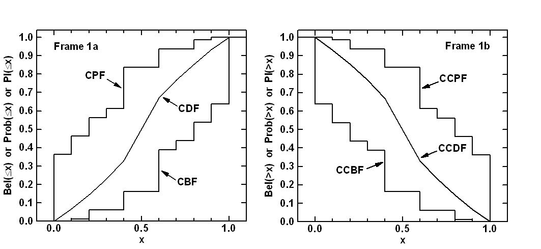
Fig. 45 Example cumulative belief and plausibility distribution functions on left; complementary cumulative belief and plausibility distribution functions on right

In evidence theory, it is not possible to specify one probability value. Instead, there is a range of values that is consistent with the evidence. The range of values is defined by belief and plausibility. Note that no statement or claim is made about one value within an interval being more or less likely than any other value.

In Dempster-Shafer evidence theory, the uncertain input variables are modeled as sets of intervals. The user assigns a basic probability assignment (BPA) to each interval, indicating how likely it is that the uncertain input falls within the interval. The BPAs for a particular uncertain input variable must sum to one. The intervals may be overlapping, contiguous, or have gaps. In Dakota, an interval uncertain variable is specified as interval_uncertain. When one defines an interval type variable in Dakota, it is also necessary to specify the number of intervals defined for each variable with iuv_num_intervals as well the basic probability assignments per interval, iuv_interval_probs, and the associated bounds per each interval, iuv_interval_bounds. Listing 43 shows the input specification for interval uncertain variables. The example has two epistemic uncertain interval variables. The first uncertain variable has three intervals and the second has two. The basic probability assignments for the first variable are 0.5, 0.1, and 0.4, while the BPAs for the second variable are 0.7 and 0.3. Note that it is possible (and often the case) to define an interval uncertain variable with only ONE interval. This means that you only know that the possible value of that variable falls within the interval, and the BPA for that interval would be 1.0. In the case we have shown, the interval bounds on the first interval for the first variable are 0.6 and 0.9, and the bounds for the second interval for the first variable are 0.1 to 0.5, etc.

Listing 43 Dakota input file for UQ example using Evidence Theory – see dakota/share/dakota/examples/users/textbook_uq_glob_evidence.in

# Dakota Input File: textbook_uq_glob_evidence.in

environment
  tabular_data
    tabular_data_file = 'textbook_uq_glob_evidence.dat'

method
  global_evidence lhs
    samples = 1000
    seed = 59334
    response_levels = 0.001 0.03 0.2 0.8 0.001 0.2 0.6 0.8
    probability_levels = 0.25 0.5 0.75 0.25 0.5 0.75
    distribution cumulative
  output verbose

variables
  continuous_interval_uncertain = 2
    num_intervals   = 3 2
    interval_probabilities  = 0.5 0.1 0.4 0.7 0.3
    lower_bounds    = 0.6 0.1 0.5 0.3 0.6
    upper_bounds    = 0.9 0.5 1.0 0.5 0.8

interface
  analysis_drivers = 'text_book'
    direct

responses
  response_functions = 2
  no_gradients
  no_hessians

Once the intervals, the BPAs, and the interval bounds are defined, the user can run an epistemic analysis by specifying the method as either global_evidence or local_evidence in the Dakota input file. Both of these methods perform Dempster-Shafer calculations: the difference is that the local method uses a local optimization algorithm to calculate the interval bounds and the global method uses either sampling or a global optimization approach to calculate an interval bound. These differences are discussed in more detail below. The intervals and their associated BPAs are then propagated through the simulation to obtain cumulative distribution functions on belief and plausibility. As mentioned above, belief is the lower bound on a probability estimate that is consistent with the evidence, and plausibility is the upper bound on a probability estimate that is consistent with the evidence.

Listing 44 shows results for the first response function obtained when running the example in Listing 43. In this example, there are 6 output intervals (as a result of the 2 interval input variables with 3 and 2 intervals, respectively). The output intervals are ordered to obtain cumulative bound functions for both belief and plausibility. The cumulative distribution function is presented for both belief (CBF) and plausibility (CPF). The CBF value is the cumulative belief corresponding to a certain output value. For example, the belief that the output value is less than or equal to 0.2 for response 1 is 0.27, and the plausibility that the output is less than or equal to 0.2 is 1 for response 1. The belief that the output value is less than 0.6217 is 0.75, while the plausbility that the output is less than 0.0806 is 0.75. The CBF and CPF may be plotted on a graph and interpreted as bounding the cumulative distribution function (CDF), which is the probability that the output is less than or equal to a certain value. The interval bounds on probability values show the value of epistemic uncertainty analysis: the intervals are usually much larger than expected, giving one a truer picture of the total output uncertainty caused by lack of knowledge or information about the epistemic input quantities.

Listing 44 Results of an Epistemic Uncertainty Quantification using Evidence Theory.

Belief and Plausibility for each response function:
Cumulative Belief/Plausibility Functions (CBF/CPF) for response_fn_1:
     Response Level  Belief Prob Level   Plaus Prob Level
     --------------  -----------------   ----------------
   1.0000000000e-03   0.0000000000e+00   0.0000000000e+00
   3.0000000000e-02   0.0000000000e+00   2.7000000000e-01
   2.0000000000e-01   2.7000000000e-01   1.0000000000e+00
   8.0000000000e-01   9.3000000000e-01   1.0000000000e+00
  Probability Level  Belief Resp Level   Plaus Resp Level
  -----------------  -----------------   ----------------
   2.5000000000e-01   2.6187288772e-01   6.2609206069e-02
   5.0000000000e-01   2.9829775860e-01   6.3736734971e-02
   7.5000000000e-01   6.2173551556e-01   8.0596931719e-02

As in other nondeterministic methods, with local_evidence or global_evidence, one can specify probability levels and response levels. If response levels are specified, the belief and plausibility function values corresponding to those response levels are calculated (see Belief Prob Level and Plaus Prob Level in the tables shown in Listing 44). Similarly, if probability levels are specified, these are first interpreted to be belief values, and the corresponding response levels are calculated (see Belief Resp Level); then they are interpreted to be plausibility values and the corresponding response levels are calculated (see Plaus Resp Level in the table in Listing 44). We have recently added the capability to support generalized reliability mappings in the evidence methods. If the user specifies a generalized reliability level, it will be first converted to a probability, then interpreted as a belief and plausibility and the corresponding response levels will be calculated. Likewise, if response levels are specified, the corresponding belief and plausibility values will be mapped to bounds on the generalized reliability levels.

To elaborate on the differences between global_evidence and local_evidence: both of these methods take the Dempster-Shafer structures specified on the inputs and calculate a resulting Dempster-Shafer structure on the outputs (e.g. a cumulative belief and plausibility function). To calculate the belief and plausibility measures, it is necessary to calculate the minimum and maximum of the response function in each “interval cell combination.” For example, in a two variable problem, if the first variable had three intervals and associated BPAs assigned and the second variable had two intervals and associated BPAs assigned, there would be 6 interval cells in total. In each of these six cells, one needs to identify a minimum and maximum value of the response function. This is easy to do if the function is monotonic in both variables, but in general it is not. We offer the capability to use local optimization methods to calculate these bounds: local_evidence allows the user to specify either sqp which is sequential quadratic programming, or nip which is a nonlinear interior point method. We also offer the capability to use global methods to assess these interval cell bounds. global_evidence allows the user to specify either lhs, which performs Latin Hypercube Sampling and takes the minimum and maximum of the samples within each cell as the bounds (no optimization is performed) or ego. In the case of ego, the efficient global optimization method is used to calculate bounds. The ego method is described in Derivative-Free Global Methods. Note that for a situation with many uncertain variables, each with a fairly complicated Dempster-Shafer structure described by many intervals, there will be a huge number of interval calls, and the overall process of performing Dempster-Shafer analysis will be extremely expensive. Reference [TIE10] provides more details about the implementation of the optimization methods to perform Dempster-Shafer calculations, as well as comparisons on test problems.

Bayesian Calibration Methods

In Bayesian calibration a “prior distribution” on a parameter is updated through a Bayesian framework involving experimental data and a likelihood function. Bayesian inference theory is best left to other sources [KOHagan01] and only a brief summary is given here. In Bayesian methods, uncertain parameters are characterized by probability density functions. These probability density functions define the permissible parameter values - the support, as well as the relative plausibility of each permissible parameter value. In the context of calibration or any inference step, the probability density function that describes knowledge before the incorporation of data is called the prior, \(f_{\boldsymbol{\Theta}}\left( \boldsymbol{\theta} \right)\).

Note: In Dakota, the prior distribution is characterized by the properties of the active uncertain variables. Correlated priors are only supported for unbounded normal, untruncated lognormal, uniform, exponential, gumbel, frechet, and weibull distributions and require a probability transformation by specifying standardized_space.

When data are available, the likelihood function describes how well each parameter value is supported by the data. Bayes Theorem [JB03], shown in (29), is used for inference: to derive the plausible parameter values, based on the prior probability density and the data \(\boldsymbol{d}\). The result is the posterior probability density function of the parameters \(f_{\boldsymbol{{\Theta |D}}}\left( \boldsymbol{{\theta |d}} \right)\). It is interpreted the same way as the prior, but includes the information derived from the data.

(29)\[{f_{\boldsymbol{\Theta |D}}}\left( \boldsymbol{\theta |d} \right) = \frac{{{f_{\boldsymbol{\Theta}}}\left( \boldsymbol{\theta} \right)\mathcal{L}\left( \boldsymbol{\theta;d} \right)}}{{{f_{\boldsymbol{D}}}\left( \boldsymbol{d} \right)}}.\]

The likelihood function is used to describe how well a model’s predictions are supported by the data. The likelihood function can be written generally as:

\[\mathcal{L}\left(\boldsymbol{{\theta ;d}} \right) = \mathcal{F}(q(\boldsymbol{\theta)} -\boldsymbol{d}),\]

where \(\boldsymbol{\theta}\) are the parameters of model quantity of interest \(q\). The form of the function \(\mathcal{F}\) can greatly influence the results. The specific likelihood function used in Dakota is based on Gaussian probability density functions. This means that we assume the difference between the model quantity (e.g. quantity of interest returned from a computer simulation) and the experimental observations are Gaussian:

(30)\[d_i = q_i(\boldsymbol{\theta}) + \epsilon_i,\]

where \(\epsilon_i\) is a random variable that can encompass both measurement errors on \(d_i\) and modeling errors associated with the simulation quantity of interest \(q_i\), for each of \(n\) observations.

If we assume that all experiments and observations are independent, then the probabilistic model defined by (30) results in a likelihood function for \(\boldsymbol{\theta}\) that is the product of \(n\) normal probability density functions:

(31)\[\mathcal{L}(\boldsymbol{{\theta};d}) = \prod_{i=1}^n \frac{1}{\sigma_d \sqrt{2\pi}} \exp \left[ - \frac{\left(d_i-q_i(\boldsymbol{{\theta}})\right)^2}{2{\sigma_d}^2} \right],\]

where \({\sigma_d}^2\) refers to the measurement error of the data, assumed constant across all data observations in this case.

We also support the more general case of a full covariance matrix, \(\boldsymbol{\Sigma_d}\), that specifies the covariance between each observation \(i\) and \(j\). In this case, the likelihood is commonly written in log form, where the log-likelihood is:

\[\label{eqn:LogLikelihood} \log{\mathcal{L}(\boldsymbol{{\theta};d})} \propto % =-0.5 {R}^{T} {\Sigma_d}^{-1} {R} -\frac{1}{2} \boldsymbol{r}^T \boldsymbol{\Sigma_d}^{-1} \boldsymbol{r},\]

where \(\boldsymbol{r}\) is the vector of residuals between the data points and the model quantity of interest, \(q(\boldsymbol{\theta})-\boldsymbol{d}\).

Dakota admits four experiment_variance_type options to specify the measurement error covariance: none for no measurement error specified (in this case, the variance is assumed to be one), scalar where a constant value \({\sigma_d}^2\) is given for all observations, diagonal where a value is specified for the diagonal elements of the covariance matrix \(\boldsymbol{\Sigma_d}\) meaning that each observation has its own measurement error but there are no cross terms, and matrix where the full covariance matrix \(\boldsymbol{\Sigma_d}\) is specified. The diagonal and matrix terms are only available for field response data. In contrast to earlier versions of Dakota, all measurement error variance should be specified with units of variance/covariance, not standard deviation.

Markov Chain Monte Carlo (MCMC) is the prototypical method used to estimate posterior parameter densities, given the observational data and the priors. There are many references that describe the basic algorithm [GRS98] and this is an active research area. MCMC algorithms may require hundreds of thousands of steps to converge, depending on dimensionality, response nonlinearity, and the desired set of posterior statistics. Since each iteration involves an evaluation of the model to obtain \(q(\boldsymbol{\theta})\), surrogate models of expensive simulations are often employed to make the MCMC process tractable.

Dakota offers five approaches for Bayesian calibration: QUESO, DREAM, GPMSA, MUQ, and WASABI. They are specified with the bayes_calibration keyword in combination with the queso, dream, gpmsa, muq, or wasabi selections, respectively. The QUESO and GPMSA methods use components from the QUESO library (Quantification of Uncertainty for Estimation, Simulation, and Optimization) developed at The University of Texas at Austin. It implements the Delayed Rejection and Adaptive Metropolis [HLMS06] (DRAM) algorithm, among others. Algorithm variants selectively combine the delayed rejection and adaptive elements. The QUESO/GPMSA capability is based on the GPMSA Matlab toolbox developed at Los Alamos National Laboratory and uses tightly integrated Gaussian process models during calibration. The Dakota implementation of QUES0/GPMSA is in a prototype stage. DREAM uses an implementation of DiffeRential Evolution Adaptive Metropolis developed by John Burkardt. The DREAM approach runs concurrent chains for global exploration, and automatically tunes the proposal covariance during the process by a self-adaptive randomized subspace sampling [VtBD+09]. MUQ uses components from the MIT Uncertainty Quantification library and also implements the Delayed Rejection and Adaptive Metropolis [HLMS06] (DRAM) algorithms, among others. The prototype WASABI method is an MCMC-free Bayesian calibration approach. QUESO/DRAM and variants are the most well-developed within Dakota.

QUESO

The QUESO library includes several sampling algorithm variants. One can use a standard Metropolis-Hastings algorithm (metropolis_hastings), adaptive Metropolis (adaptive_metropolis) for adapting the proposal covariance during the sampling, delayed rejection (delayed_rejection) for backtracking from sample rejections, the full DRAM (dram) which involves both delayed rejection and adaptive Metropolis, or a multi-level algorithm (multilevel). This last option is not yet production-ready in Dakota.

With any choice of sampling algorithm, one may manually set the burn in period for the MCMC chain with burn_in_samples. If a sub_sampling_period is specified, the MCMC chain is further filtered such that only the sample at the beginning of each period is in the final MCMC chain. The sub_sampling_period should therefore be greater than or equal to the correlation length of the samples.

With the QUESO method, one may run the MCMC sampling on the simulation model directly. However, if the model is expensive, use of a surrogate (emulator) model is recommended. Options include a Gaussian process, a polynomial chaos expansion, or a stochastic collocation expansion.

The proposal covariance refers to the covariance structure of a multivariate normal distribution, which governs sample generation in the chain. One may specify proposal_covariance, followed by prior (the default), values, filename, or derivatives. With the prior setting, the proposal covariance will be set to the variance of the prior distributions of the parameters being calibrated. When specifying the proposal covariance with input file values or from a separate file, the user may specify only the diagonals of the covariance matrix or the full covariance matrix.

The derivatives option will use derivatives from the simulation or emulator model to form or approximate the Hessian of the misfit function (the negative log likelihood). Especially when derivative information is available inexpensively (e.g. from an emulator), the derivative-based proposal covariance forms a more accurate proposal distribution, resulting in lower rejection rates and faster chain mixing. When using an emulator, the derivative-based proposal covariance should be updated periodically using the posterior_adaptive specification. This will add simulation truth evaluations in areas of high-likelihood to the emulator training data, thus refining the Hessian. For more detail about derivative-based formulations involving the misfit Hessian, refer to Proposal Densities.

An additional control for QUESO is to perform a logit transformation (logit_transform) which performs an internal variable transformation from bounded domains to unbounded domains.

This option can be helpful when regions of high posterior density exist in the corners of a multi-dimensional bounded domain. In these cases, it may be difficult to generate feasible samples from the proposal density, and transformation to unbounded domains may greatly reduce sample rejection rates.

The pre_solve option will perform a deterministic gradient-based optimization before the MCMC sampling to get a good starting point for the chain. This pre-solve seeks to maximize the log-posterior (the log-likelihood minus the log-prior) to identify the maximum a posteriori probability point, also called the MAP point. The Markov Chain will then start at the MAP point, which can circumvent a lot of initial searching for high posterior probability points. The pre-solve option can be used with an emulator or with no emulator.

Credible and prediction intervals will be calculated if probability_levels is specified. Credible intervals propagate uncertainties in parameter density information to the quantity of interest and quantify how well the model fits the provided data, while prediction intervals propagate both parameter and experimental measurement uncertainties and contain the next experimental or simulated observation with the specified probability. Further details can be found in [Smi13]. If probability_levels is specified, credible intervals will always be calculated. Prediction intervals will only be calculated if experiment_variance_type is also specified in the responses block. By specifying posterior_stats, information-theoretic metrics may be calculated using the posterior distribution of parameters. If the kl_divergence option is selected, the Kullback-Leibler Divergence will be calculated between the posterior and the prior distributions such that

\[D_{KL} = \int {f_{\boldsymbol{\Theta |D}}}\left( \boldsymbol{\theta |d} \right) \log \frac{ {f_{\boldsymbol{\Theta |D}}}\left( \boldsymbol{\theta |d} \right) } {{f_{\boldsymbol{\Theta}}}\left( \boldsymbol{\theta} \right)} d\boldsymbol{\theta}.\]

This quantity represents the amount of information gained about the parameters during the Bayesian update. Further details regarding the calculation and use of \(D_{KL}\) can be found in Information Theoretic Tools.

DREAM

For the DREAM method, one can define the number of chains (minimum 3) used with the chains specification. The total number of generations per chain in DREAM is the number of samples divided by the number of chains. The number of chains randomly selected to be used in the crossover each time a crossover occurs is crossover_chain_pairs. There is an extra adaptation during burn-in, in which DREAM estimates a distribution of crossover probabilities that favors large jumps over smaller ones in each of the chains. Normalization is required to ensure that all of the input dimensions contribute equally. In this process, a discrete number of candidate points for each crossover value is generated, which can be specified with num_cr. The gr_threshold control is the convergence tolerance for the Gelman-Rubin statistic, which governs the convergence of the multiple chain process. The integer jump_step forces a long jump every jump_step generations. For more details about these parameters, refer to [VtBD+09]. Credible and prediction intervals can be calculated by specifying probability_levels, and statistics regarding the posterior may be calculated by specifying posterior_stats, as described in QUESO.

GPMSA

Core to GPMSA is the construction of a Gaussian process emulator from simulation runs collected at various settings of input parameters. The emulator is a statistical model of the system response, and it is used to incorporate the observational data to improve system predictions and constrain or calibrate the unknown parameters. The GPMSA code draws heavily on the theory developed in the seminal Bayesian calibration paper by Kennedy and O’Hagan [KOHagan01]. The particular approach developed by the Los Alamos group, and implemented in QUESO and therefore Dakota, is provided in [HGWR08]. It includes an embedded discrepancy model and the ability to estimate various hyper-parameters of the Gaussian process, observation error model, and discrepancy model. Dakota’s gpmsa capability is an experimental prototype with a number of limitations.

MUQ

MUQ is the MIT Uncertainty Quantification library. See https://bitbucket.org/mituq/muq2/src/master/ and https://mituq.bitbucket.io/index.html for additional documentation. Dakota currently exposes four MCMC approaches from MUQ: Metropolis-Hastings, Adaptive Metropolis, Delayed Rejection, and Delayed-Rejection Adaptive Metropolis. Dakota’s MUQ integration is preliminary, anticipated to extend to use MUQ components for Hamiltonian Monte Carlo and Langevin-based sampling. MUQ is an experimental Dakota capability, and as such, it is not turned on by default, and must be explicitly enabled when compiling Dakota.

WASABI

WASABI differs from the other Bayesian approaches in that it is not an MCMC-based approach. Instead, it is based on the idea of “consistent Bayes” which is outlined in [BJW17]. This approach to stochastic inference uses measure-theoretic principles to construct a probability measure or density on model parameters that is consistent with the model and the data. The idea is that the probability measure on the parameters, when “pushed-foward” through the computational model, will give results that match the probability measure on the observational data.

We use a similar notation as with the Bayesian methods, but the interpretation is different here. The goal is to identify the posterior density on the parameters, \(\pi_{post}({\theta})\), which is equal to the prior density on the parameters times a ratio. The numerator of the ratio, \(\pi_{D}^{obs}\), describes the relative likelihood that the output of the model corresponds to the observed data \({D}\): this is the density of the data evaluated at the model output. \(q(\boldsymbol{\theta})\) refers to the model output. \(\pi_{D}^{q_{prior}}\) refers to the push-forward of the prior through the model and represents a forward propagation of uncertainty.

\[\pi_{post}(\boldsymbol{\theta})=\pi_{prior}(\boldsymbol{\theta})\frac{\pi_{D}^{obs}(q(\boldsymbol{\theta}))}{\pi_{D}^{q_{prior}}(q(\boldsymbol{\theta}))}. \label{eq:consistentBayesEq}\]

The Fundamentals section of the main Bayesian Methods theory page has more detail about the assumptions and mathematical foundations for this method. Note a major difference in interpretation of the posterior results with respect to a standard Bayesian approach: In a standard Bayesian approach, the posterior reflects an updated state of information about the prior distribution on parameter values induced by the observational data. In consistent Bayes, the posterior reflects a stochastic mapping of parameter values such that the posterior parameters, when pushed-forward through the model, give results that are consistent with the density of the observational data. Dakota’s wasabi keyword is a prototype capability.

Feature Comparison

Table 9 compares the options available with the QUESO, DREAM, GPMSA, MUQ, and WASABI implementations in Dakota.

Table 9 Capabilities of Bayesian methods in Dakota
Capability	QUESO	MUQ	GPMSA	DREAM	WASABI
Prior Distributions	Any continuous variable type	Any continuous variable type	Any continuous variable type	Uniform only	Uniform only
Inference Type	MCMC with DR, AM, DRAM, or MH	MCMC with DR, AM, DRAM, or MH	MCMC with DR, AM, DRAM, or MH	MCMC with Differential Evolution Adaptive Metropolis	MCMC- free interval analysis
Can use PCE/SC Emulator	Yes	Yes	Yes	Yes	Yes
Can use GP Emulator	Yes	Yes	Yes (required)	Yes	Yes
Likelihood-based adaptive emulator update	Yes	No	No	No	No
Initialize with MAP pre-solve	Yes	Yes	No	No	No
Proposal covariance options	prior, user, derivative-based	n/a	prior, user	n/a	n/a
Can calibrate error covariance multipliers	Yes	Yes	Yes (internal)	Yes	No
Supports standardized space	Yes	Yes	Yes	Yes	Yes
Logit transform	Yes	Yes	Yes	No	No
Posterior export	samples	samples	samples	samples	samples, density

Bayesian Calibration Example

To run a QUESO-based Bayesian calibration in Dakota, create a Dakota input file such as the one shown in Listing 45. Here, the QUESO DRAM (delayed rejection adaptive metropolis) solver is selected. The number of samples = 1000 indicates how many points to generate in the acceptance chain 3. This example uses the mod_cantilever algebraic model, so an emulator is not warranted. The proposal covariance used has diagonal element values of 1.e6 and 0.1. Two credible and prediction intervals will be calculated for each model output: a 5/95 interval and a 10/90 interval. The calibration terms in the responses section refers to the number of outputs that will be used in the calibration process: in this case, it is just two. The calibration data file has the observational data: in this case, it is a freeform file (e.g. no header or annotation) with ten experiments. For each experiment, there are two experiment values, one for stress and one for displacement, followed by two variance values for the error associated with that experiment for each quantity of interest.

Listing 45 Dakota input file for Bayesian calibration

method
  bayes_calibration queso
    chain_samples = 10000 seed = 348
    dram  # | delayed_rejection | adaptive_metropolis | metropolis_hastings
    proposal_covariance
      values 1.0e6 1.0e-1
        diagonal
    logit_transform         # default is off
    probability_levels 0.05 0.1
                       0.05 0.1
    posterior_stats kl_divergence

variables
  uniform_uncertain 2
    upper_bounds  1.e8 10.0
    lower_bounds 1.e6 0.1
    initial_point 2.85e7 2.5
    descriptors 'E' 'w'
  continuous_state 4
    initial_state 3 40000 500 1000
    descriptors 't' 'R' 'X' 'Y'

interface
  analysis_drivers = 'mod_cantilever'
    direct

responses
  calibration_terms = 2
  calibration_data_file = 'dakota_cantilever_queso.withsigma.dat'
    freeform
    num_experiments = 10
    variance_type = 'scalar' # read 2 scalar sigmas in each row
  descriptors = 'stress' 'displacement'
  no_gradients
  no_hessians

When the input file shown in Listing 45 is run, Dakota will run the MCMC algorithm and generate a posterior sample of \(\boldsymbol{\theta}\) in accordance with Bayes Theorem (29) and the likelihood function (31). Dakota’s final output summary reports an evaluation count summary and the best sample point visited during the MCMC process as measured by maximum posterior probability (an estimate of the MAP point). The final output also summarizes the moments of the posterior samples from the chain (e.g. mean of the chain, standard deviation of the chain samples, etc.), as well as the credible and prediction intervals for each model output.

Auxilliary output is also generated to a directory called QuesoDiagnostics/ in the directory from which Dakota is run. The file display_sub0.txt contains diagnostic information regarding the MCMC process. The Matlab files contained in the QuesoDiagnostics/ directory contain the chain files. The files to load in Matlab are raw_chain.m or filtered_chain.m, containing the full chain or the filtered chain values of the parameters 4. In addition, the accepted chain values that Dakota generates are written to a file in the run directory called (by default) dakota_mcmc_tabular.dat. The first columns of this file are the posterior values of the input variables. If burn_in or sub_sampling_period are specified, the filtered acceptance chain is instead written to the file dakota_mcmc_tabular.dat. This file contains the posterior values of the filtered MCMC chain, as well as the values of state variables and the resulting model responses. Finally, if one wants to see the likelihood of each point, specifying verbose output in the method section will result in the likelihoods being printed.

Chain Diagnostics

The convergence of the chain produced by MCMC may require many thousands of steps, if not millions, as discussed earlier in this section. Assessing the convergence of MCMC chains is an active area of research, and the implementation of metrics for chain convergence is undergoing active development in Dakota, and can be triggered during a Bayesian calibration study through the use of the keyword chain_diagnostics.

Note

As of Dakota 6.10, confidence_intervals is the only diagnostic implemented.

Suppose \(g\) is a function that represents some characteristic (e.g. moment) of an underlying distribution, such as the mean or variance. Then under the standard assumptions of an MCMC chain, the true value can be approximated by taking the ensemble mean over the MCMC chain. The confidence interval for the true moment calculated using the asymptotically valid interval estimator is given by [FJ10]

\[\bar{g}_{n} \pm t_{*} \frac{\hat{\sigma}_{n}}{\sqrt{n}},\]

where \(\bar{g}_{n}\) is the estimated moment (i.e. mean or variance), \(t_{*}\) is the Student’s \(t\)-value for the 95th quantile, \(n\) is the MCMC chain length, and \(\hat{\sigma}_{n}\) is an estimate of the standard error whose square is obtained using batch means estimation. To obtain the estimate \(\hat{\sigma}_{n}\), the Markov chain produced during calibration is broken up into “batches,” the sample moment is calculated for each batch, and \(\hat{\sigma}_{n}\) is subsequently obtained as an unbiased estimate of the standard deviation in the moment calculations over the batches. The confidence intervals produced are 95% confidence intervals, and they are calculated for the mean and variance (first and second moments) for each parameter and each response. Further details regarding the default settings for these calculations can be found in Chain Diagnostics.

Confidence intervals may be used as a chain diagnostic by setting fixed-width stopping rules [RKA18]. For example, if the interval width is below some threshold value, that may indicate that enough samples have been drawn. Common choices for the threshold value include:

Fixed width: \(\epsilon\)
Relative magnitude: \(\epsilon \| \bar{g}_{n} \|\)
Relative standard deviation: \(\epsilon \| \hat{\sigma}_{n} \|\)

If the chosen threshold is exceeded, samples may need to be increased, say by 10%, and the diagnostics reevaluated for signs of chain convergence. Furthermore, if output is set to debug, the sample moment for each batch (for each parameter and response) is output to the screen. The user can then analyze the convergence of these batch means in order to deduce whether the MCMC chain has converged.

Calibrating the Observation Error Model

As discussed in Calibration data import, Dakota accepts user information on the covariance \(\Sigma_d\) among observation errors and includes this in the likelihood formulation:

\[\log{\mathcal{L}(\boldsymbol{{\theta};d})} \propto % =-0.5 {R}^{T} {\Sigma_d}^{-1} {R} -\frac{1}{2} \boldsymbol{r}^T \boldsymbol{\Sigma_d}^{-1} \boldsymbol{r}.\]

In some cases, it can be helpful to fine tune the assumptions in this covariance during the calibration process. Dakota supports calibrating one or more multipliers on the blocks of the error covariance. So if \(\Sigma_d\) is block diagonal such that \(\Sigma_d = \mbox{diag}({\Sigma_d}_1, ..., {\Sigma_d}_N)\), we instead formulate as \(\Sigma_d = \mbox{diag}(m_1{\Sigma_d}_1, ..., m_P{\Sigma_d}_P)\) and calibrate the multipliers \(m_i\) as hyper-parameters in the Bayesian inference process.

The supported modes for calibrating observation error multipliers are shown in Table 10: one, per_experiment, per_response, and both. Here, the two major blocks denote two experiments, while the inner blocks denote five response groups (two scalar, three field). The priors on the hyper-parameters \(m_i\) are taken to be inverse gamma distributions, with mean and mode approximately 1.0 and standard deviation approximately 0.1.

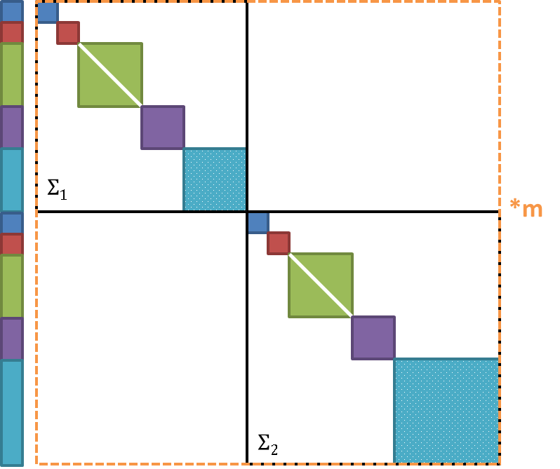
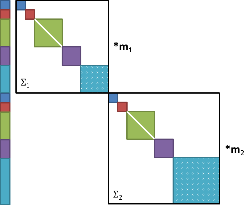
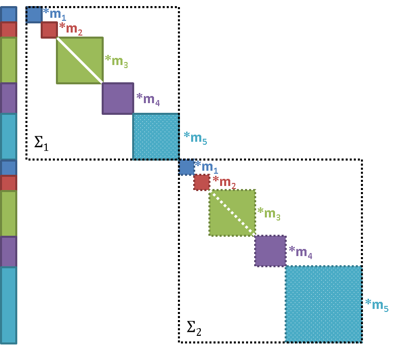
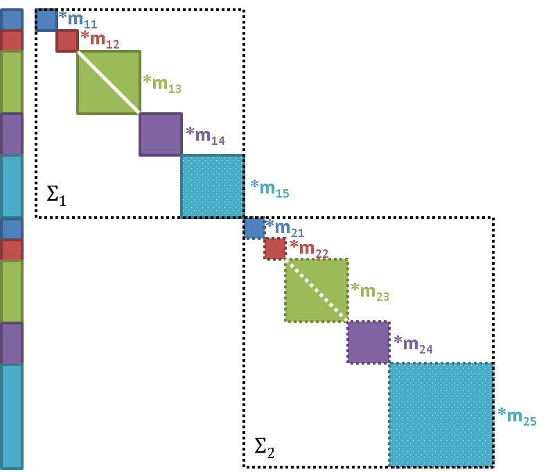
Table 10 Calibrating observational error covariance multipliers: (a) one multiplier on whole user-provided covariance structure, (b) multiplier per-experiment, (c) multiplier per-response, and (d) both.

Scaling and Weighting of Residuals

Dakota’s scaling options, described in Optimization with User-specified or Automatic Scaling, can be used on Bayesian calibration problems, using the primary_scales keyword, to scale the residuals between the data points and the model predictions, if desired. Additionally, Bayesian calibration residuals-squared can be weighted via the weights specification. Neither set of weights nor scales are adjusted during calibration. When response scaling is active, it is applied after error variance weighting and before weights application. The calibration_terms documentation has more detail about weighting and scaling of the residual terms.

Model Evidence

In some situations, there are multiple models that may represent a phenomenon and the user is left with the task to determine which is most appropriate given the available data. In this case, Bayesian model selection may help. Suppose that the user has a set of models, \(\mathcal{M}\)=\(M_1,M_2...M_m\) from which to choose. In the Bayesian setting, the parameters of each of these models may be updated according to Bayes’ rule:

\[\pi_{post}(\boldsymbol{\theta_i}|D,M_i)=\pi_{prior}(\boldsymbol{\theta_i}|M_i)\frac{\pi(D|\boldsymbol{\theta_i},M_i)}{\pi(D|M_i)}\]

where the dependence on the model has been made explicit. The denominator is used as the likelihood of a specific model of interest in a version of Bayes’ rule which calculates the posterior model plausibility as:

(32)\[\pi_{post}(M_i|D)=\pi_{prior}(M_i)\frac{\pi(D|M_i)}{\pi(D)}\]

In this equation, the posterior model probability given the data is also referred to as model plausibility. The prior model plausibility, \(\pi(M_i)\), is usually taken to be uniform, meaning equally likely for all models, but it does not have to be. \(\pi(D)\) is a normalizing factor such that the sum of all model plausibilities is 1. In this context, model selection involves choosing the model with the highest posterior model plausibility. Model evidence is defined as the likelihood in (32), denoted by \(\pi(D|M_i)\). Model evidence is determined by averaging the likelihood of its model parameters over all possible values of the model parameters, according to their prior distributions. It is also called the marginal likelihood of the model. Model evidence is defined as:

(33)\[\pi(D|M_i)=\int \pi(D|\boldsymbol{\theta_i},M_i)\pi_{prior}(\boldsymbol{\theta_i}|M_i)d \boldsymbol{\theta_i}\]

There are many ways to calculate model evidence. There are currently two methods implemented in Dakota. The user first specifies model_evidence, then either mc_approx and/or laplace_approx depending on the method(s) used to calculate model evidence.

Monte Carlo approximation. This involves sampling from the prior distribution of the parameters, calculating the corresponding likelihood values at those samples, and estimating the integral given in Eq. (33) by brute force. The number of samples used in the sampling of the integral is determined by evidence_samples. Although this method is easy, it is not efficient because each sample of the prior density requires an evaluation of the simulation model to compute the corresponding likelihood. Additionally, many prior samples will have very low (near zero) likelihood, so millions of samples may be required for accurate computation of the integral.
Laplace approximation. This approach is based on the Laplace approximation, as outlined in [Was00]. It has the assumption that the posterior distribution is nearly Gaussian, which is not always a safe assumption. Then, with maximum a posteriori (MAP) point \(\hat{\boldsymbol{\theta}}\), the Laplace approximation of model evidence is:

\[\int \pi(D|\boldsymbol{\theta_i},M_i)\pi_{prior}(\boldsymbol{\theta_i}|M_i)d \boldsymbol{\theta_i} \approx \pi(D|\hat{\boldsymbol{\theta}},M_i)\pi(\hat{\boldsymbol{\theta}}|M_i)(2\pi)^{N_i/2}{\|\det(H(\hat{\boldsymbol{\theta}}))\|}^{-1/2}\]

where \(N_i\) is the number of unknown parameters in the i-th model and \(H\) is the negative Hessian of the log-posterior evaluated at the MAP point \(\hat{\boldsymbol{\theta}}\). Therefore, this implementation only requires the evaluation of the model likelihood and the Hessian of the log-posterior density at the MAP point.

Model Discrepancy

Whether in a Bayesian setting or otherwise, the goal of model calibration is to minimize the difference between the observational data \(d_i\) and the corresponding model response \(q_i(\boldsymbol{\theta})\). In the presence of scenario or configuration variables \(x\), Eq. (30) can be modified,

\[d_i(x) = q_i\left(\boldsymbol{\theta}, x\right) + \epsilon_i,\]

with the ensuing equations of the likelihood and Bayes’ Theorem updated likewise. The configuration variables represent experimental settings, such as temperature or pressure, that may vary between experiments.

However, it is often the case that the agreement between the data and the model after calibration is not sufficiently close. This is generally attributed to model form or structural error, and can be corrected to some extent with the use of model discrepancy. The Kennedy and O’Hagan [KOHagan01] formulation takes the form

\[d_i(x) = q_i\left(\boldsymbol{\theta}, x\right) + \delta_i(x) + \epsilon_i,\]

where \(\delta_i(x)\) represents the model discrepancy. For scalar responses, the model discrepancy is only a function of the configuration variables. Furthermore, one discrepancy model is calculated for each observable \(d_i\), \(i = 1, \ldots, n\), yielding \(\delta_1, \ldots, \delta_n\). For field responses, a single, global \(\delta\) is a function of the configuration variables as well as the independent field coordinates, which are usually points in time or space. The construction of the model discrepancy in cases with mixed scalar and field responses has not been tested.

The current implementation of the model discrepancy capability in Dakota serves as a post-processing mechanism after the completion of a Bayesian update. If model_discrepancy is specified in the input file, Dakota will perform the Bayesian update as detailed in the section above, and then begin the process of approximating \(\delta\). For each scalar observable \(d_i\) and for each configuration \(x_j\),

\[\delta_i \left( x_j \right) = d_i \left( x_j \right) - q_i \left(\boldsymbol{\theta}^*, x_j \right),\]

where \(\boldsymbol{\theta}^*\) is the average of the calibrated posterior distribution of the model parameters. The \(i^{th}\) discrepancy function will be built over the computed \(\delta_i \left( x_j \right)\), \(j = 1, \ldots, m\). For field observable \(d\), the discrepancy is calculated for each independent field coordinate \(t_{i}\) and for each configuration \(x_{j}\),

\[\delta(t_{i}, x_{j}) = d(t_{i}, x_{j}) - q(\boldsymbol{\theta}^{*}, t_{i}, x_{j}).\]

The global discrepancy function is then built over the computed \(\delta(t_{i}, x_{j})\), \(i = 1, \ldots, n\), \(j = 1, \ldots, m\). For simplicity in future notation, we let \(\delta_{i}(x_i) = \delta(t_i, x_i)\).

The field discrepancy function is built using a Gaussian process regression model with a quadratic trend function. If instead the responses are scalars, more options for the regression model are available. Within the Dakota input file, the user may specify the discrepancy_type to be either a Gaussian process or polynomial regression model with the gaussian_process or polynomial commands, respectively. Additionally, the order of the trend function may be selected using the correction_order command and choosing one of constant, linear, or quadratic. Any specifications using these keywords will apply to all \(\delta_i\). By default, Dakota will build a Gaussian process discrepancy model with a quadratic trend function. Information regarding how polynomial and Gaussian process models are built can be found in Linear, Quadratic, and Cubic Polynomial Models and Kriging/Gaussian-Process Spatial Interpolation Models, respectively.

The user may specify new “prediction” configurations at which the corrected model should be calculated. For each response and for each new configuration, \(q_i(\boldsymbol{\theta}, x_{k,new}) + \delta_i(x_{k,new})\) will be computed. The prediction configurations can be specified in one of three ways. If num_prediction_configs is included, Dakota will uniformly distribute the indicated number of prediction configurations throughout the domain of the configuration variable that is given in the variables block of the input file. Alternatively, the user may explicitly list desired prediction configuration locations within the input file following the prediction_configs keyword, or in an external file to be read in with the import_prediction_configs option. If none of these three options is selected, Dakota will automatically calculate corrected model predictions at ten configurations in the scalar response case, with the predictions spread uniformly in the configuration variable domain. In the case of field responses, corrected model predictions are calculated for each value of the input configuration variable(s).

Calculations corresponding to each prediction configuration and to each observable will be output to tabular files. The responses from the discrepancy model itself is output to dakota_discrepancy_tabular.dat. Those from the corrected model are output to dakota_corrected_tabular.dat. The user may specify the output file names for the discrepancy and corrected model tabular files using the export_discrepancy_file and export_corrected_model_file keywords, respectively.

Variance information corresponding to each specified configuration location and for each observable is also computed. In a prediction setting for scalar responses, the variance calculated from the discrepancy model is additively combined with the variance information provided with the experimental data, such that

(34)\[\Sigma_{total,i}(x) = \Sigma_{\delta, i}(x) + \sigma^{2}_{exp,i} I\]

for each observable \(i\). Further details of how the variance \(\Sigma_{\delta,i}(x)\) is computed for Gaussian process and polynomial regression models can be found in Model Discrepancy. The experimental variance provided for parameter calibration may vary for the same observable from experiment to experiment, thus \(\sigma^{2}_{exp,i}\) is taken to be the maximum variance given for each observable. That is,

\[\sigma^2_{exp,i} = \max_{j} \sigma^2_{i}(x_j),\]

where \(\sigma^2_{i}(x_j)\) is the variance provided for the \(i^{th}\) observable \(d_i\), computed or measured with the configuration variable \(x_j\).

When each corrected model value \(q_i(\boldsymbol{\theta}^{*}, x_{k, new}) + \delta_i(x_{k,new})\) is considered, the variance calculated via (34) provides a prediction interval, similar to those described in QUESO. Including \(\sigma^{2}_{exp,i}\) in the variance calculation accounts for the uncertainty in the model predictions that arise due to uncertainties in the calibration data. These prediction variances are output to the file dakota_discrepancy_variance_tabular.dat by default. The name of this file can be modified using the export_corrected_variance_file keyword in the input script. If the response is a field, the variance information written to this file is the variance of the Gaussian process alone. Future work includes calculation of combined experimental variance and discrepancy model variance for field responses.

Note

Additional details and an illustrative example of these calculations are given in Scalar Responses Example and Field Responses Example.

Bayesian Experimental Design

The goal of experimental design is to add observational data to the Bayesian update that informs model parameters and reduces their uncertainties. In Bayesian approaches, data from physical experiments is typically used to calibrate a model. However, another common practice is to use responses or output from a high-fidelity model as “truth data” in place of experimental data in a low-fidelity model calibration. This can be done in with a single Bayesian calibration, or it can be done iteratively with the use of experimental design, where an initial set of high-fidelity runs is augmented sequentially to find the next “best” high-fidelity design point at which to run the high-fidelity model to add to the calibration data. The low-fidelity posterior parameter distribution is then updated again using Bayesian calibration. The mutual information is used as the selection criterion to guide the process of high-fidelity data acquisition.

In Dakota, design conditions, such as temperature or spatial location, can be specified using so-called configuration variables. The design selection algorithm implemented in Dakota uses a user-specified high-fidelity code to produce the “experimental” or observational data that is used in the calibration of the desired low-fidelity model. The high-fidelity model is dependent only upon the design or configuration variables while the low-fidelity model depends on both the design variables and uncertain model parameters.

An example Dakota input file that implements this Bayesian experimental design algorithm is shown in Listing 46. Note that there are three model blocks, one describing the model hierarchy and one each for the high-fidelity and low-fidelity models. There are two variables, interface, and responses blocks such that each model has its own specifications. The low-fidelity variables block contains information about both the design variables, which are specified with continuous_state, and the parameters to be updated via Bayes’ Theorem (29), which are specified using one of the aleatory uncertain variable types discussed in Section Uncertain Variables. In the high-fidelity variables block, only the continuous_state parameters are included. The specifications of the design variables should be consistent in both blocks. Each interface block should point to the appropriate high- or low-fidelity code, and the responses blocks should contain consistent details about the responses from each code. For example, both of the models should return the same number of calibration_terms.

Listing 46 Dakota input file for Bayesian Experimental Design.

environment
  tabular_data

method,
       bayes_calibration queso
          dram
    seed = 34785
          chain_samples = 500
          experimental_design
          initial_samples = 2
    num_candidates = 2
    import_candidate_points_file = 'dakota_bayes_expdesign.cand.dat'
    freeform
    #ksg2
    max_hifi_evaluations = 1
          model_pointer = 'HIERARCH'

model,
  id_model = 'HIERARCH'
  variables_pointer = 'ALL_VARS'
  surrogate ensemble
    ordered_model_fidelities = 'LF' 'HF'

model,
        id_model = 'LF'
        single
          interface_pointer = 'lofi_IF'
        variables_pointer = 'ALL_VARS'
        responses_pointer = 'lofi_resp'

model,
        id_model = 'HF'
        single
          interface_pointer = 'hifi_IF'
        variables_pointer = 'CONFIG_VARS'
        responses_pointer = 'hifi_resp'

variables,
  id_variables = 'ALL_VARS'
        continuous_state = 1
    upper_bounds = 70
          lower_bounds = 10
        uniform_uncertain = 3
    upper_bounds   0.06   0     260
    lower_bounds   0  -8  0

variables,
  id_variables = 'CONFIG_VARS'
  active state
  continuous_state = 1
          upper_bounds = 70
          lower_bounds = 10

interface,
        id_interface = 'hifi_IF'
        analysis_drivers = 'expdesign_high'
          fork

interface,
        id_interface = 'lofi_IF'
        analysis_drivers = 'expdesign_low'
          fork

responses,
  id_responses = 'lofi_resp'
        calibration_terms = 1
  no_gradients
  no_hessians

responses,
  id_responses = 'hifi_resp'
  calibration_terms = 1
  calibration_data_file = 'dakota_bayes_expdesign.dat'
    freeform
    num_config_variables = 1
    num_experiments = 2
    experiment_variance_type = 'none'
  no_gradients
  no_hessians

The mutual information experimental design algorithm is selected by specifying bayes_calibration, queso, and experimental_design within the method block of the input file, and the first model block should contain the hierarchical specification of the surrogate keyword. The algorithm starts by performing a Bayesian calibration using a number of data points, specified in Dakota by initial_samples. These initial data points can be pulled from external data using the calibration_data_file keyword in the high-fidelity responses block. In this case, num_config_variables should be specified and set to the number of configuration variables captured in the variables blocks. Furthermore, for use in Bayesian experimental design, calibration_data_file should contain the configuration variables and the corresponding high-fidelity model responses. Scalar variance information may be included for the calibration data through the use of the experiment_variance_type or simulation_variance command within the high-fidelity responses block. The former is applied to any user-provided data, such as through the calibration_data_file keyword, while the latter applies only to those high-fidelity model responses produced by the high-fidelity code run by Dakota. If the number of points taken from this file is less than initial_samples, or if no such file is provided, Latin Hypercube Sampling is used to draw samples of the design space, and the high-fidelity model is run at these points to supplement the user-specified data. After this initial calibration, a set of design conditions (i.e. configuration variables) of size num_candidates is proposed. Users may specify these candidate points through the import_candidate_points_file command. Again, if the number of points in this file is less than num_candidates, or if no such file is provided, Latin Hypercube Sampling is used to draw samples of the design space.

From these candidate designs, that which maximizes the mutual information with respect to the low-fidelity model parameters is deemed “optimal.” The mutual information is approximated using the low-fidelity model and a \(k\)-nearest neighbor algorithm, as detailed in [LSWF16]. This optimal design is used in the high-fidelity model to create a new observation, which is appended to the initial data. This updated data is used to recalculate the Bayesian posterior, and the process repeats until one of three stopping criteria are met. Multiple optimal designs may be selected concurrently by specifying batch_size in the input script. These designs are selected using the greedy algorithm described in detail in Experimental Design. In this case, the high-fidelity model is run at all batch-selected optimal designs before the Bayesian posterior is recalculated with the updated data for an ensuing iteration of the experimental design algorithm.

There are two algorithms that may be used to calculate the mutual information, both of which are derived in [KStogbauerG04]. The first algorithm discussed therein is used as the default algorithm within Dakota; the second may be selected by including the keyword ksg2 in the Dakota input script. Furthermore, the user may choose to include, during the computation of the mutual information, a stochastic error term on the low-fidelity model responses. This is done by specifying simulation_variance in the responses block corresponding to the low-fidelity model. See Experimental Design for more information regarding the implementation of the mutual information calculations.

There are three criteria by which this algorithm is considered complete. The user may specify max_hifi_evaluations, which limits the number of high-fidelity model simulations Dakota will run. Note that this does not include any simulations needed to perform the initial Bayesian calibration of the low-fidelity model parameters. Alternatively, if the change in the mutual information from one iteration to the next is sufficiently small or if all candidate points have been exhausted, the algorithm will terminate.

Progress of the algorithm will be reported to the screen with the rest of the Dakota output. Furthermore, a summary of the algorithm’s results, including, for each iteration, the optimal design, the mutual information, and the corresponding high-fidelity model response, can be found in the file experimental_design_output.txt.

One-at-a-time Implementation

There may be some applications for which the high-fidelity model must be run independently of Dakota. This algorithm may still be implemented in this case, however, it requires some extra work by the user to ensure that the high-fidelity model information is properly communicated to Dakota, as a “dummy” high-fidelity model code must be supplied to Dakota. The data to be used in the initial Bayesian calibration should be gathered from the high-fidelity model or physical experiment and imported via the calibration_data_file in the high-fidelity responses block, and extra care should be taken to ensure that initial_samples matches the number of experiments in this file. It is also best, for this use-case, to use import_candidate_points_file, with num_candidates exactly matching the number of candidate points in the file.

By setting max_hifi_evaluations to zero, Dakota will run the initial calibration of the low-fidelity model, select the optimal design (or multiple optimal designs when batch_size is greater than 1) from those provided in import_candidate_points_file, and exit without running the “dummy” high-fidelity model code. The selected design(s) will be output to the screen, as well as to experimental_design_output.txt, as detailed above. The high-fidelity model may then be run offline with the newly selected design point(s).

The user must update calibration_data_file with the new high-fidelity data when it becomes available, as well as remove the previously selected design point(s) from import_candidate_points_file. Within the Dakota input file, initial_samples, num_experiments, and num_candidates should be correspondingly updated. Dakota may then be run again to yield the next optimal experimental design(s). It should be noted that the stopping criteria will not be automatically evaluated by Dakota when one-at-a-time implementation is used. The user must determine when the algorithm should be terminated.

Uncertainty Quantification Usage Guidelines

The choice of uncertainty quantification method depends on how the input uncertainty is characterized, the computational budget, and the desired output accuracy. The recommendations for UQ methods are summarized in Table 11 and are discussed in the remainder of the section.

Table 11 Guidelines for UQ method selection.
Method	Desired Problem	Applicable Methods
Classification	Characteristics
Sampling	nonsmooth, multimodal response functions;	sampling (Monte Carlo or LHS)
	response evaluations are relatively inexpensive
Local	smooth, unimodal response functions;	local_reliability (MV, AMV/AMV\(^2\),
reliability	larger sets of random variables;	AMV +/AMV\(^2\)+, TANA, FORM/SORM)
	estimation of tail probabilities
Global	smooth or limited nonsmooth response;	global_reliability
reliability	multimodal response; low dimensional;
	estimation of tail probabilities
Adaptive	smooth or limited nonsmooth response;	importance_sampling,
Sampling	multimodal response; low dimensional;	gpais, adaptive_sampling,
	estimation of tail probabilities	pof_darts
Stochastic	smooth or limited nonsmooth response;	polynomial_chaos,
expansions	multimodal response; low dimensional;	stoch_collocation
	estimation of moments or moment-based metrics
Epistemic	uncertainties are poorly characterized	interval: local_interval_est,
		global_interval_est, sampling;
		BPA: local_evidence, global_evidence
Mixed UQ	some uncertainties are poorly characterized	nested UQ (IVP, SOP, DSTE) with epistemic
		outer loop and aleatory inner loop, sampling

Sampling Methods

Sampling-based methods are the most robust uncertainty techniques available, are applicable to almost all simulations, and possess rigorous error bounds; consequently, they should be used whenever the function is relatively inexpensive to compute and adequate sampling can be performed. In the case of terascale computational simulations, however, the number of function evaluations required by traditional techniques such as Monte Carlo and Latin hypercube sampling (LHS) quickly becomes prohibitive, especially if tail statistics are needed.

Alternatively, one can apply the traditional sampling techniques to a surrogate function approximating the expensive computational simulation (see Surrogate-Based Uncertainty Quantification). However, if this approach is selected, the user should be aware that it is very difficult to assess the accuracy of the results obtained. Unlike the case of surrogate-based local minimization (see Surrogate-Based Local Minimization), there is no simple pointwise calculation to verify the accuracy of the approximate results. This is due to the functional nature of uncertainty quantification, i.e. the accuracy of the surrogate over the entire parameter space needs to be considered, not just around a candidate optimum as in the case of surrogate-based local. This issue especially manifests itself when trying to estimate low probability events such as the catastrophic failure of a system.

Reliability Methods

Local reliability methods (e.g., MV, AMV/AMV\(^2\), AMV+/AMV\(^2\)+, TANA, and FORM/SORM) are more computationally efficient in general than the sampling methods and are effective when applied to reasonably well-behaved response functions; i.e., functions that are smooth, unimodal, and only mildly nonlinear. They can be used to provide qualitative sensitivity information concerning which uncertain variables are important (with relatively few function evaluations), or compute full cumulative or complementary cumulative response functions (with additional computational effort). Since they rely on gradient calculations to compute local optima (most probable points of failure), they scale well for increasing numbers of random variables, but issues with nonsmooth, discontinuous, and multimodal response functions are relevant concerns. In addition, even if there is a single MPP and it is calculated accurately, first-order and second-order integrations may fail to accurately capture the shape of the failure domain. In these cases, adaptive importance sampling around the MPP can be helpful. Overall, local reliability methods should be used with some care and their accuracy should be verified whenever possible.

An effective alternative to local reliability analysis when confronted with nonsmooth, multimodal, and/or highly nonlinear response functions is efficient global reliability analysis (EGRA). This technique employs Gaussian process global surrogate models to accurately resolve the failure domain and then employs multimodal adaptive importance sampling to resolve the probabilities. For relatively low dimensional problems (i.e, on the order of 10 variables), this method displays the efficiency of local reliability analysis with the accuracy of exhaustive sampling. While extremely promising, this method is still relatively new and is the subject of ongoing refinements as we deploy it to additional applications.

Adaptive Sampling Methods

There are now a number of methods in Dakota which are tailored to estimating tail probabilities. These methods include both standard importance sampling and Gaussian Process Adaptive Importance Sampling, as well as adaptive sampling and the POF-darts method. These methods are suitable for smooth or limited non-smooth responses, and work well in low dimensions. GPAIS and POF-darts utilize a Gaussian process surrogate model.

Stochastic Expansions Methods

The next class of UQ methods available in Dakota is comprised of stochastic expansion methods (polynomial chaos and stochastic collocation), which are general purpose techniques provided that the response functions possess finite second order moments. Further, these methods capture the underlying functional relationship between a key response metric and its random variables, rather than just approximating statistics such as mean and standard deviation. This class of methods parallels traditional variational methods in mechanics; in that vein, efforts are underway to compute rigorous error bounds of the approximations produced by the methods. Another strength of these methods is their potential use in a multiphysics environment as a means to propagate the uncertainty through a series of simulations while retaining as much information as possible at each stage of the analysis. The current challenge in the development of these methods, as for other global surrogate-based methods, is effective scaling for large numbers of random variables. Recent advances in adaptive collocation and sparsity detection methods address some of the scaling issues for stochastic expansions.

Epistemic Uncertainty Quantification Methods

The final class of UQ methods available in Dakota are focused on epistemic uncertainties, or uncertainties resulting from a lack of knowledge. In these problems, the assignment of input probability distributions when data is sparse can be somewhat suspect. One approach to handling epistemic uncertainties is interval analysis (local_interval_est and global_interval_est), where a set of intervals on inputs, one interval for each input variable, is mapped to a set of intervals on outputs. To perform this process efficiently, optimization methods can be used. Another related technique is Dempster-Shafer theory of evidence (Dakota methods local_evidence and global_evidence), where multiple intervals per input variable (which can be overlapping, contiguous, or disjoint) are propagated, again potentially using optimization methods. The choice between local or global optimization methods for interval computation is governed by the same issues described in Optimization Usage Guidelines.

Mixed Aleatoric and Epistemic Methods

For problems with a mixture of epistemic and aleatoric uncertainties, it is desirable to segregate the two uncertainty types within a nested analysis, allowing stronger probabilistic inferences for the portion of the problem where they are appropriate. In this nested approach, an outer epistemic level selects realizations of epistemic parameters (augmented variables) and/or realizations of random variable distribution parameters (inserted variables). These realizations define the objective probabilistic analysis to be performed on the inner aleatoric level. In the case where the outer loop involves propagation of subjective probability, the nested approach is known as second-order probability and the study generates a family of CDF/CCDF respresentations known as a “horse tail” plot. In the case where the outer loop is an interval propagation approach (local_interval_est or global_interval_est), the nested approach is known as interval-valued probability (see also Nested Models) . In the case where the outer loop is an evidence-based approach (local_evidence or global_evidence), the approach generates epistemic belief and plausibility bounds on aleatory statistics.

1: Orthogonal polynomial selections also exist for discrete probability distributions, but are not yet supported in Dakota.
2: Identical support range; weight differs by at most a constant factor.
3: If delayed rejection is active, the number of simulation evaluations will typically be higher due to backtracking.
4: The full chain will be output in cases of adaptive posterior refinement or proposal updating, since these use cases access the entire acceptance chain to identify refinement data or restarting points, respectively.

Video Resources

Title	Link	Resources
Uncertainty Quantification		Slides / Exercises
Sampling

Uncertainty Quantification

Overview

Summary of Dakota UQ Methods

Variables and Responses for UQ

Sampling Methods

Uncertainty Quantification Example using Sampling Methods

Incremental Sampling

Principal Component Analysis

Wilks-based Sample Sizes

Double Sided Tolerance Interval Equivalent Normal Distribution

Reliability Methods

Local Reliability Methods

Method mapping

Global Reliability Methods

Uncertainty Quantification Examples using Reliability Analysis

Mean-value Reliability with Textbook

FORM Reliability with Lognormal Ratio

Stochastic Expansion Methods

Uncertainty Quantification Examples using Stochastic Expansions

Polynomial Chaos Expansion for Rosenbrock

Uncertainty Quantification Example using Stochastic Collocation

Importance Sampling Methods

Importance Sampling Method based on Reliability Approach

Gaussian Process Adaptive Importance Sampling Method

Adaptive Sampling Methods

Adaptive sampling based on surrogates

Adaptive sampling based on dart throwing

Epistemic Nondeterministic Methods

Interval Methods for Epistemic Analysis

Dempster-Shafer Theory of Evidence

Bayesian Calibration Methods

QUESO

DREAM

GPMSA

MUQ

WASABI

Feature Comparison

Bayesian Calibration Example

Chain Diagnostics

Calibrating the Observation Error Model

Scaling and Weighting of Residuals

Model Evidence

Model Discrepancy

Bayesian Experimental Design

One-at-a-time Implementation

Uncertainty Quantification Usage Guidelines

Video Resources

Exceptional service in the national interest