Dakota Input File

• Input File Formatting
• Models
• Variables
• Interfaces
• Responses
• Inputs to Dakota
• Dakota Input Spec

Note

If you are looking for video resources on Dakota’s input file format, click here.

There are six specification blocks that may appear in Dakota input files. These are identified in the input file using the following keywords: variables, interface, responses, model, method, and environment. While, these keyword blocks can appear in any order in a Dakota input file, there is an inherent relationship that ties them together. The simplest form of that relationship is shown in Fig. 32:

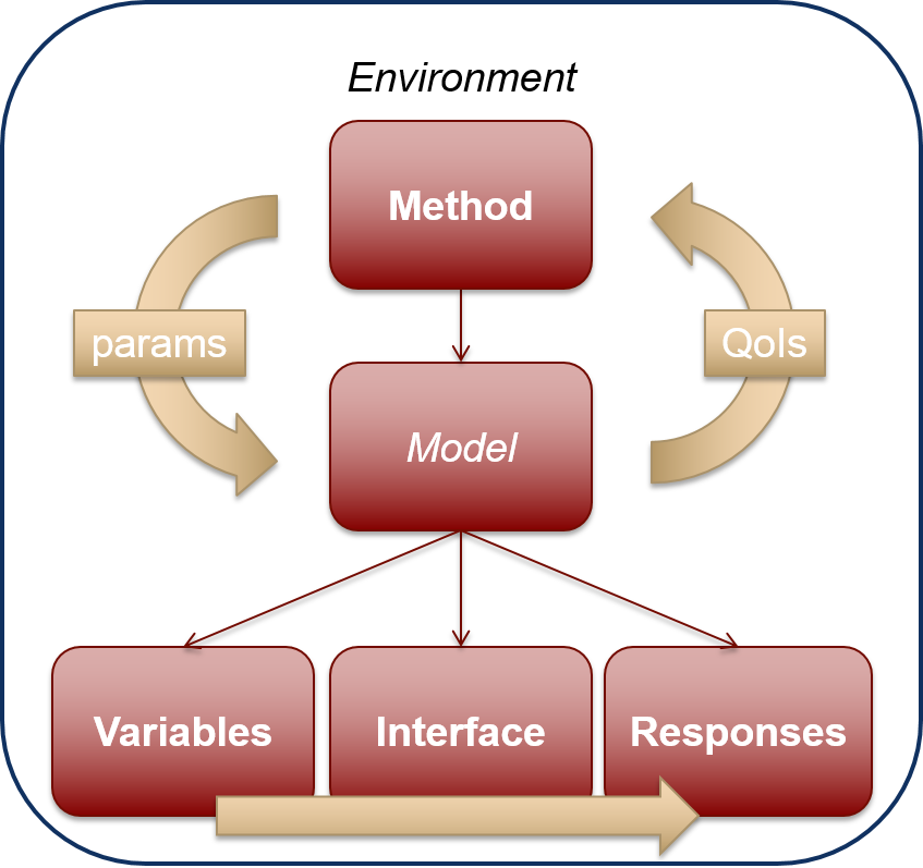
Fig. 32 Relationship between the six blocks, for a simple study.

It can be summarized as follows: In each iteration of its algorithm, a method block requests a variables-to-responses mapping from its model, which the model fulfills through an interface.

Listing 24 Rosenbrock 2-D parameter study example: the Dakota input file.

# Dakota Input File: rosen_multidim.in
# Usage:
#   dakota -i rosen_multidim.in -o rosen_multidim.out > rosen_multidim.stdout

environment
  tabular_data
    tabular_data_file = 'rosen_multidim.dat'

method
  multidim_parameter_study
    partitions = 8 8

model
  single

variables
  continuous_design = 2
    lower_bounds     -2.0     -2.0
    upper_bounds      2.0      2.0
    descriptors       'x1'     "x2"

interface
  analysis_drivers = 'rosenbrock'
    direct

responses
  response_functions = 1
  no_gradients
  no_hessians

As a concrete example, a simple Dakota input file, rosen_multidim.in, is shown above in Listing 24, for a two-dimensional parameter study on Rosenbrock’s function. This input file will be used to describe the basic format and syntax used in all Dakota input files.

Note

To see the results of this study and more, consult the Examples section.

Note

While most Dakota analyses satisfy the relationship where a single method runs a single model, advanced cases are possible.

The first block of the input file is the environment block. This keyword block is used to specify the general Dakota settings such as Dakota’s graphical output (via the graphics flag) and the tabular data output (via the tabular data keyword). In advanced cases, it also identifies the top method pointer that will control the Dakota study. The environment block is optional, and at most one such block can appear in a Dakota input file.

The method block of the input file specifies which iterative method Dakota will employ and associated method options. The keyword multidim parameter study in Listing 24 calls for a multidimensional parameter study, while the keyword partitions specifies the number of intervals per variable (a method option). In this case, there will be eight intervals (nine data points) evaluated between the lower and upper bounds of both variables (bounds provided subsequently in the variables section), for a total of 81 response function evaluations. At least one method block is required, and multiple blocks may appear in Dakota input files for advanced studies.

The model block of the input file specifies the model that Dakota will use. A model provides the logical unit for determining how a set of variables is mapped through an interface into a set of responses when needed by an iterative method. In the default case, the model allows one to specify a single set of variables, interface, and responses. The model block is optional in this simple case. Alternatively, it can be explicitly defined as in Listing 24, where the keyword single specifies the use of a single model in the parameter study. If one wishes to perform more sophisticated studies such as surrogate-based analysis or optimization under uncertainty, the logical organization specified in the model block becomes critical in informing Dakota on how to manage the different components of such studies, and multiple model blocks are likely needed.

The variables block of the input file specifies the number, type, and characteristics of the parameters that will be varied by Dakota. The variables can be classified as design variables, uncertain variables, or state variables. Design variables are typically used in optimization and calibration, uncertain variables are used in UQ and sensitivity studies, and state variables are usually fixed. In all three cases, variables can be continuous or discrete, with discrete having real, integer, and string subtypes. The variables section shown in Listing 24 specifies that there are two continuous design variables. The sub-specifications for continuous design variables provide the descriptors “x1” and “x2” as well as lower and upper bounds for these variables. The information about the variables is organized in column format for readability. So, both variables x1 and x2 have a lower bound of -2.0 and an upper bound of 2.0. At least one variables block is required, and multiple blocks may appear in Dakota input files for advanced studies.

The interface block of the input file specifies the simulation code that will be used to map variables into responses as well as details on how Dakota will pass data to and from that code. In this example, the keyword direct is used to indicate the use of a function linked directly into Dakota, and data is passed directly between the two. The name of the function is identified by the analysis driver keyword. Alternatively, fork or system executions can be used to invoke instances of a simulation code that is external to Dakota as explained here and here. In this case, data is passed between Dakota and the simulation via text files. At least one interface block is required, and multiple blocks may appear in Dakota input files for advanced studies.

The responses block of the input file specifies the types of data that the interface will return to Dakota. They are categorized primarily according to usage. Objective functions are used in optimization, calibration terms in calibration, and response functions in sensitivity analysis and UQ. For the example shown in Listing 24, the assignment response functions = 1 indicates that there is only one response function. The responses block can include additional information returned by the interface. That includes constraints and derivative information. In this example, there are no constraints associated with Rosenbrock’s function, so the keywords for constraint specifications are omitted. The keywords no gradients and no hessians indicate that no derivatives will be provided to the method; none are needed for a parameter study. At least one responses block is required, and multiple blocks may appear in Dakota input files for advanced studies.

Video Resources

Title	Link	Resources
Input File Format
Input Syntax / Building Blocks		Slides / Exercises