Advanced Methods
Overview
A variety of “meta-algorithm” capabilities have been developed in order to provide a mechanism for employing individual iterators and models as reusable components within higher-level solution approaches. This capability allows the use of existing iterative algorithm and computational model software components as building blocks to accomplish more sophisticated studies, such as hybrid, multistart, Pareto, or surrogate-based minimization. Further multi-component capabilities are enabled by the model recursion capabilities described in the page Models with specific examples in the page Advanced Models.
Hybrid Minimization
In the hybrid minimization method (keyword: hybrid), a sequence of
minimization methods are applied to find an optimal design point. The
goal of this method is to exploit the strengths of different
minimization algorithms through different stages of the minimization
process. Global/local optimization hybrids (e.g., genetic algorithms
combined with nonlinear programming) are a common example in which the
desire for a global optimum is balanced with the need for efficient
navigation to a local optimum. An important related feature is that the
sequence of minimization algorithms can employ models of varying
fidelity. In the global/local case, for example, it would often be
advantageous to use a low-fidelity model in the global search phase,
followed by use of a more refined model in the local search phase.
The specification for hybrid minimization involves a list of method
identifier strings, and each of the corresponding method specifications
has the responsibility for identifying the model specification (which
may in turn identify variables, interface, and responses specifications)
that each method will use (see the Dakota Reference
Manual Keyword Reference and the example discussed below).
Currently, only the sequential hybrid approach is available. The
embedded and collaborative approaches are not fully functional
at this time.
In the sequential hybrid minimization approach, a sequence of
minimization methods is invoked in the order specified in the Dakota
input file. After each method completes execution, the best solution or
solutions from that method are used as the starting point(s) for the
following method. The number of solutions transferred is defined by how
many that method can generate and how many the user specifies with the
individual method keyword final_solutions. For example, currently
only a few of the global optimization methods such as genetic algorithms
(e.g. moga and coliny_ea) and sampling methods return multiple
solutions. In this case, the specified number of solutions from the
previous method will be used to initialize the subsequent method. If the
subsequent method cannot accept multiple input points (currently only a
few methods such as the genetic algorithms in JEGA allow multiple input
points), then multiple instances of the subsequent method are generated,
each one initialized by one of the optimal solutions from the previous
method. For example, if LHS sampling were run as the first method and
the number of final solutions was 10 and the DOT conjugate gradient was
the second method, there would be 10 instances of dot_frcg started,
each with a separate LHS sample solution as its initial point. Method
switching is governed by the separate convergence controls of each
method; that is, each method is allowed to run to its own internal
definition of completion without interference. Individual method
completion may be determined by convergence criteria (e.g.,
convergence_tolerance) or iteration limits (e.g.,
max_iterations).
Listing 55 shows a Dakota input file that specifies a
sequential hybrid optimization method to solve the “textbook”
optimization test problem. The textbook_hybrid_strat.in file
provided in dakota/share/dakota/examples/users starts with a
coliny_ea solution which feeds its best point into a
coliny_pattern_search optimization which feeds its best point into
optpp_newton. While this approach is overkill for such a simple
problem, it is useful for demonstrating the coordination between
multiple sub-methods in the hybrid minimization algorithm.
The three optimization methods are identified using the method_list
specification in the hybrid method section of the input file. The
identifier strings listed in the specification are ‘GA’ for genetic
algorithm, ‘PS’ for pattern search, and ‘NLP’ for nonlinear
programming. Following the hybrid method keyword block are the three
corresponding method keyword blocks. Note that each method has a tag
following the id_method keyword that corresponds to one of the
method names listed in the hybrid method keyword block. By following the
identifier tags from method to model and from model to
variables, interface, and responses, it is easy to see the
specification linkages for this problem. The GA optimizer runs first and
uses model ‘M1’ which includes variables ‘V1’, interface
‘I1’, and responses ‘R1’. Note that in the specification,
final_solutions=1, so only one (the best) solution is returned from
the GA. However, it is possible to change this to final_solutions=5
and get five solutions passed from the GA to the Pattern Search (for
example). Once the GA is complete, the PS optimizer starts from the best
GA result and again uses model ‘M1’. Since both GA and PS are
nongradient-based optimization methods, there is no need for gradient or
Hessian information in the ‘R1’ response keyword block. The NLP
optimizer runs last, using the best result from the PS method as its
starting point. It uses model ‘M2’ which includes the same ‘V1’
and ‘I1’ keyword blocks, but uses the responses keyword block
‘R2’ since the full Newton optimizer used in this example
(optpp_newton) needs analytic gradient and Hessian data to perform
its search.
dakota/share/dakota/examples/users/textbook_hybrid_strat.in# Dakota Input File: textbook_hybrid_strat.in
environment
top_method_pointer = 'HS'
method
id_method = 'HS'
hybrid sequential
method_pointer_list = 'GA' 'PS' 'NLP'
method
id_method = 'GA'
coliny_ea
seed = 1234
population_size = 5
model_pointer = 'M1'
final_solutions = 1
output verbose
method
id_method = 'PS'
coliny_pattern_search
stochastic
initial_delta = 0.1
seed = 1234
variable_tolerance = 1e-4
solution_target = 1.e-10
exploratory_moves
basic_pattern
model_pointer = 'M1'
output verbose
method
id_method = 'NLP'
optpp_newton
gradient_tolerance = 1.e-12
convergence_tolerance = 1.e-15
model_pointer = 'M2'
output verbose
model
id_model = 'M1'
single
interface_pointer = 'I1'
variables_pointer = 'V1'
responses_pointer = 'R1'
model
id_model = 'M2'
single
interface_pointer = 'I1'
variables_pointer = 'V1'
responses_pointer = 'R2'
variables
id_variables = 'V1'
continuous_design = 2
initial_point 0.6 0.7
upper_bounds 5.8 2.9
lower_bounds 0.5 -2.9
descriptors 'x1' 'x2'
interface
id_interface = 'I1'
analysis_drivers = 'text_book'
direct
responses
id_responses = 'R1'
objective_functions = 1
no_gradients
no_hessians
responses
id_responses = 'R2'
objective_functions = 1
analytic_gradients
analytic_hessians
Multistart Local Minimization
A simple, heuristic, global minimization technique is to use many local
minimization runs, each of which is started from a different initial
point in the parameter space. This is known as multistart local
minimization. This is an attractive method in situations where multiple
local optima are known or expected to exist in the parameter space.
However, there is no theoretical guarantee that the global optimum will
be found. This approach combines the efficiency of local minimization
methods with a user-specified global stratification (using a specified
starting_points list, a number of specified random_starts, or
both; see the Dakota Reference Manual Keyword Reference for
additional specification details). Since solutions for different
starting points are independent, parallel computing may be used to
concurrently run the local minimizations.
An example input file for multistart local optimization on the
“quasi_sine” test function (see quasi_sine_fcn.C in
dakota_source/test) is shown in
Listing 56. The method keyword
block in the input file contains the keyword multi_start, along with
the set of starting points (3 random and 5 listed) that will be used for
the optimization runs. The other keyword blocks in the input file are
similar to what would be used in a single optimization run.
dakota/share/dakota/examples/users/qsf_multistart_strat.in# Dakota Input File: qsf_multistart_strat.in
environment
top_method_pointer = 'MS'
method
id_method = 'MS'
multi_start
method_pointer = 'NLP'
random_starts = 3 seed = 123
starting_points = -0.8 -0.8
-0.8 0.8
0.8 -0.8
0.8 0.8
0.0 0.0
method
id_method = 'NLP'
## (DOT requires a software license; if not available, try
## conmin_mfd or optpp_q_newton instead)
dot_bfgs
variables
continuous_design = 2
lower_bounds -1.0 -1.0
upper_bounds 1.0 1.0
descriptors 'x1' 'x2'
interface
analysis_drivers = 'quasi_sine_fcn'
fork #asynchronous
responses
objective_functions = 1
analytic_gradients
no_hessians
The quasi_sine test function has multiple local minima, but there is
an overall trend in the function that tends toward the global minimum at
\((x1,x2)=(0.177,0.177)\). See [GE00] for more
information on this test function.
Listing 57 shows the results
summary for the eight local optimizations performed. From the five
specified starting points and the 3 random starting points (as
identified by the x1, x2 headers), the eight local optima (as
identified by the x1*, x2* headers) are all different and only
one of the local optimizations finds the global minimum.
   <<<<< Results summary:
      set_id             x1             x2            x1*            x2*         obj_fn
           1           -0.8           -0.8  -0.8543728666  -0.8543728666   0.5584096919
           2           -0.8            0.8  -0.9998398719    0.177092822    0.291406596
           3            0.8           -0.8    0.177092822  -0.9998398719    0.291406596
           4            0.8            0.8   0.1770928217   0.1770928217   0.0602471946
           5              0              0  0.03572926375  0.03572926375  0.08730499239
           6  -0.7767971993  0.01810943539  -0.7024118387  0.03572951143   0.3165522387
           7  -0.3291571008  -0.7697378755   0.3167607374  -0.4009188363   0.2471403213
           8   0.8704730469   0.7720679005    0.177092899   0.3167611757  0.08256082751
Pareto Optimization
The Pareto optimization method (keyword: pareto_set ) is one of three
multiobjective optimization capabilities discussed in
Section Multiobjective Optimization.
In the Pareto optimization method, multiple sets of multiobjective
weightings are evaluated. The user can specify these weighting sets in
the method keyword block using a list, a number of , or both (see the
Dakota Reference Manual Keyword Reference for additional
specification details).
Dakota performs one multiobjective optimization problem for each set of multiobjective weights. The collection of computed optimal solutions form a Pareto set, which can be useful in making trade-off decisions in engineering design. Since solutions for different multiobjective weights are independent, parallel computing may be used to concurrently execute the multiobjective optimization problems.
Listing 59 shows the results
summary for the Pareto-set optimization method. For the four
multiobjective weighting sets (as identified by the w1, w2,
w3 headers), the local optima (as identified by the x1, x2
headers) are all different and correspond to individual objective
function values of (\(f_1,f_2,f_3\)) = (0.0,0.5,0.5),
(13.1,-1.2,8.16), (532.,33.6,-2.9), and (0.125,0.0,0.0) (note: the
composite objective function is tabulated under the obj_fn header).
The first three solutions reflect exclusive optimization of each of the
individual objective functions in turn, whereas the final solution
reflects a balanced weighting and the lowest sum of the three
objectives. Plotting these (\(f_1,f_2,f_3\)) triplets on a
3-dimensional plot results in a Pareto surface (not shown), which is
useful for visualizing the trade-offs in the competing objectives.
dakota/share/dakota/examples/users/textbook_pareto_strat.in# Dakota Input File: textbook_pareto_strat.in
environment
top_method_pointer = 'PS'
method
id_method = 'PS'
pareto_set
method_pointer = 'NLP'
weight_sets =
1.0 0.0 0.0
0.0 1.0 0.0
0.0 0.0 1.0
0.333 0.333 0.333
method
id_method = 'NLP'
## (DOT requires a software license; if not available, try
## conmin_mfd or optpp_q_newton instead)
dot_bfgs
model
single
variables
continuous_design = 2
initial_point 0.9 1.1
upper_bounds 5.8 2.9
lower_bounds 0.5 -2.9
descriptors 'x1' 'x2'
interface
analysis_drivers = 'text_book'
direct
responses
objective_functions = 3
analytic_gradients
no_hessians
   <<<<< Results summary:
      set_id             w1             w2             w3             x1             x2         obj_fn
           1              1              0              0   0.9996554048    0.997046351 7.612301561e-11
           2              0              1              0            0.5            2.9           -1.2
           3              0              0              1            5.8 1.12747589e-11           -2.9
           4          0.333          0.333          0.333            0.5   0.5000000041       0.041625
Mixed Integer Nonlinear Programming (MINLP)
Many nonlinear optimization problems involve a combination of discrete and continuous variables. These are known as mixed integer nonlinear programming (MINLP) problems. A typical MINLP optimization problem is formulated as follows:
where \(\mathbf{d}\) is a vector whose elements are integer values. In situations where the discrete variables can be temporarily relaxed (i.e., noncategorical discrete variables, see Section Discrete Design Variables, the branch-and-bound algorithm can be applied. Categorical variables (e.g., true/false variables, feature counts, etc.) that are not relaxable cannot be used with the branch and bound method. During the branch and bound process, the discrete variables are treated as continuous variables and the integrality conditions on these variables are incrementally enforced through a sequence of optimization subproblems. By the end of this process, an optimal solution that is feasible with respect to the integrality conditions is computed.
Dakota’s branch and bound method (keyword: branch_and_bound) can
solve optimization problems having either discrete or mixed
continuous/discrete variables. This method uses the parallel
branch-and-bound algorithm from the PEBBL software
package [EPH09] to generate a series of optimization
subproblems (“branches”). These subproblems are solved as continuous
variable problems using any of Dakota’s nonlinear optimization
algorithms (e.g., DOT, NPSOL). When a solution to a branch is feasible
with respect to the integrality constraints, it provides an upper bound
on the optimal objective function, which can be used to prune branches
with higher objective functions that are not yet feasible. Since
solutions for different branches are independent, parallel computing may
be used to concurrently execute the optimization subproblems.
PEBBL, by itself, targets the solution of mixed integer linear programming (MILP) problems, and through coupling with Dakota’s nonlinear optimizers, is extended to solution of MINLP problems. In the case of MILP problems, the upper bound obtained with a feasible solution is an exact bound and the branch and bound process is provably convergent to the global minimum. For nonlinear problems which may exhibit nonconvexity or multimodality, the process is heuristic in general, since there may be good solutions that are missed during the solution of a particular branch. However, the process still computes a series of locally optimal solutions, and is therefore a natural extension of the results from local optimization techniques for continuous domains. Only with rigorous global optimization of each branch can a global minimum be guaranteed when performing branch and bound on nonlinear problems of unknown structure.
In cases where there are only a few discrete variables and when the discrete values are drawn from a small set, then it may be reasonable to perform a separate optimization problem for all of the possible combinations of the discrete variables. However, this brute force approach becomes computationally intractable if these conditions are not met. The branch-and-bound algorithm will generally require solution of fewer subproblems than the brute force method, although it will still be significantly more expensive than solving a purely continuous design problem.
Example MINLP Problem
As an example, consider the following MINLP problem [ES99]:
This problem is a variant of the textbook test problem described in Section Additional Examples Textbook. In addition to the introduction of two integer variables, a modified value of \(1.4\) is used inside the quartic sum to render the continuous solution a non-integral solution.
Figure 45 shows the sequence of branches generated for this problem. The first optimization subproblem relaxes the integrality constraint on parameters \(x_{5}\) and \(x_{6}\), so that \(0 \leq x_{5} \leq 4\) and \(0 \leq x_{6} \leq 4\). The values for \(x_{5}\) and \(x_{6}\) at the solution to this first subproblem are \(x_{5}=x_{6}=1.4\). Since \(x_{5}\) and \(x_{6}\) must be integers, the next step in the solution process “branches” on parameter \(x_{5}\) to create two new optimization subproblems; one with \(0 \leq x_{5} \leq 1\) and the other with \(2 \leq x_{5} \leq 4\). Note that, at this first branching, the bounds on \(x_{6}\) are still \(0 \leq x_{6} \leq 4\). Next, the two new optimization subproblems are solved. Since they are independent, they can be performed in parallel. The branch-and-bound process continues, operating on both \(x_{5}\) and \(x_{6}\) , until a optimization subproblem is solved where \(x_{5}\) and \(x_{6}\) are integer-valued. At the solution to this problem, the optimal values for \(x_{5}\) and \(x_{6}\) are \(x_{5}=x_{6}=1\).
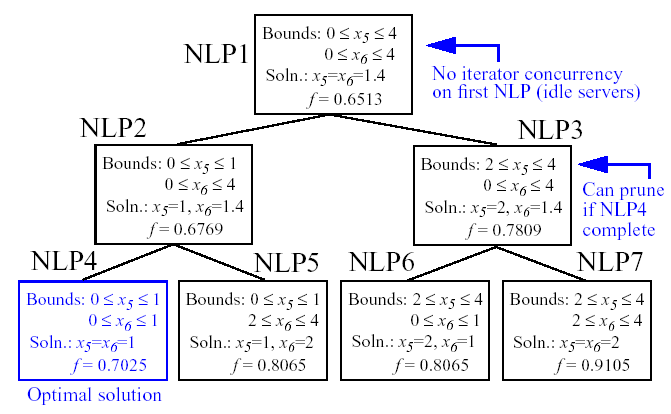
Fig. 53 Branching history for example MINLP optimization problem.
In this example problem, the branch-and-bound algorithm executes as few as five and no more than seven optimization subproblems to reach the solution. For comparison, the brute force approach would require 25 optimization problems to be solved (i.e., five possible values for each of \(x_{5}\) and \(x_{6}\) ).
In the example given above, the discrete variables are integer-valued. In some cases, the discrete variables may be real-valued, such as \(x \in \{0.0,0.5,1.0,1.5,2.0\}\). The branch-and-bound algorithm is restricted to work with integer values. Therefore, it is up to the user to perform a transformation between the discrete integer values from Dakota and the discrete real values that are passed to the simulation code (see Section:ref:Discrete Design Variables <variables:design:ddv>). When integrality is not being relaxed, a common mapping is to use the integer value from Dakota as the index into a vector of discrete real values. However, when integrality is relaxed, additional logic for interpolating between the discrete real values is needed.
Surrogate-Based Minimization
Surrogate models approximate an original, high fidelity “truth” model, typically at reduced computational cost. In Dakota, several surrogate model selections are possible, which are categorized as data fits, multifidelity models, and reduced-order models, as described in Section Models Surrogate. In the context of minimization (optimization or calibration), surrogate models can speed convergence by reducing function evaluation cost or smoothing noisy response functions. Three categories of surrogate-based minimization are discussed in this chapter:
Trust region-managed surrogate-based local minimization, with data fit surrogate, multifidelity models, or reduced-order models.
Surrogate-based global minimization, where a single surrogate is built (and optionally iteratively updated) over the whole design space.
Efficient global minimization: nongradient-based constrained and unconstrained optimization and nonlinear least squares based on Gaussian process models, guided by an expected improvement function.
Surrogate-Based Local Minimization
In the surrogate-based local minimization method (keyword:
surrogate_based_local) the minimization algorithm operates on a
surrogate model instead of directly operating on the computationally
expensive simulation model. The surrogate model can be based on data
fits, multifidelity models, or reduced-order models, as described in
Section Models Surrogate. Since the surrogate
will generally have a limited range of accuracy, the surrogate-based
local algorithm periodically checks the accuracy of the surrogate model
against the original simulation model and adaptively manages the extent
of the approximate optimization cycles using a trust region approach.
Refer to the Dakota Reference Manual Keyword Reference for algorithmic guidelines and details on iterate acceptance, merit function formulations, convergence assessment, and constraint relaxation.
SBO with Data Fits
When performing SBO with local, multipoint, and global data fit surrogates, it is necessary to regenerate or update the data fit for each new trust region. In the global data fit case, this can mean performing a new design of experiments on the original high-fidelity model for each trust region, which can effectively limit the approach to use on problems with, at most, tens of variables. Figure 46 displays this case. However, an important benefit of the global sampling is that the global data fits can tame poorly-behaved, non-smooth, discontinuous response variations within the original model into smooth, differentiable, easily navigable, and easily navigated surrogates. This allows SBO with global data fits to extract the relevant global design trends from noisy simulation data.
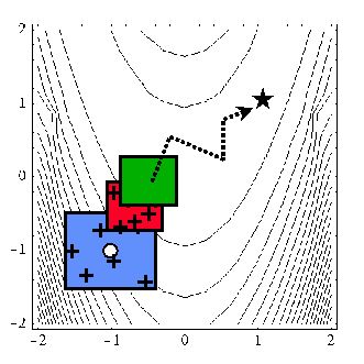
Fig. 54 SBO iteration progression for global data fits.
When enforcing local consistency between a global data fit surrogate and a high-fidelity model at a point, care must be taken to balance this local consistency requirement with the global accuracy of the surrogate. In particular, performing a correction on an existing global data fit in order to enforce local consistency can skew the data fit and destroy its global accuracy. One approach for achieving this balance is to include the consistency requirement within the data fit process by constraining the global data fit calculation (e.g., using constrained linear least squares). This allows the data fit to satisfy the consistency requirement while still addressing global accuracy with its remaining degrees of freedom. Embedding the consistency within the data fit also reduces the sampling requirements. For example, a quadratic polynomial normally requires at least \((n+1)(n+2)/2\) samples for \(n\) variables to perform the fit. However, with an embedded first-order consistency constraint at a single point, the minimum number of samples is reduced by \(n+1\) to \((n^2+n)/2\).
In the local and multipoint data fit cases, the iteration progression will appear as in Fig. 55. Both cases involve a single new evaluation of the original high-fidelity model per trust region, with the distinction that multipoint approximations reuse information from previous SBO iterates. Like model hierarchy surrogates, these techniques scale to larger numbers of design variables. Unlike model hierarchy surrogates, they generally do not require surrogate corrections, since the matching conditions are embedded in the surrogate form (as discussed for the global Taylor series approach above). The primary disadvantage to these surrogates is that the region of accuracy tends to be smaller than for global data fits and multifidelity surrogates, requiring more SBO cycles with smaller trust regions. More information on the design of experiments methods is available in Section Dace, and the data fit surrogates are described in Section Models Surrogate Datafit.
Listing 60 shows a Dakota input file
that implements surrogate-based optimization on Rosenbrock’s function.
The first method keyword block contains the SBO keyword
surrogate_based_local, plus the commands for specifying the trust
region size and scaling factors. The optimization portion of SBO, using
the CONMIN Fletcher-Reeves conjugate gradient method, is specified in
the following keyword blocks for method, model, variables,
and responses. The model used by the optimization method specifies
that a global surrogate will be used to map variables into responses (no
interface specification is used by the surrogate model). The global
surrogate is constructed using a DACE method which is identified with
the ‘SAMPLING’ identifier. This data sampling portion of SBO is
specified in the final set of keyword blocks for method, model,
interface, and responses (the earlier variables
specification is reused). This example problem uses the Latin hypercube
sampling method in the LHS software to select 10 design points in each
trust region. A single surrogate model is constructed for the objective
function using a quadratic polynomial. The initial trust region is
centered at the design point \((x_1,x_2)=(-1.2,1.0)\), and extends
\(\pm 0.4\) (10% of the global bounds) from this point in the
\(x_1\) and \(x_2\) coordinate directions.
dakota/share/dakota/examples/users/rosen_opt_sbo.in# Dakota Input File: rosen_opt_sbo.in
environment
tabular_data
tabular_data_file = 'rosen_opt_sbo.dat'
top_method_pointer = 'SBLO'
method
id_method = 'SBLO'
surrogate_based_local
model_pointer = 'SURROGATE'
method_pointer = 'NLP'
max_iterations = 500
trust_region
initial_size = 0.10
minimum_size = 1.0e-6
contract_threshold = 0.25
expand_threshold = 0.75
contraction_factor = 0.50
expansion_factor = 1.50
method
id_method = 'NLP'
conmin_frcg
max_iterations = 50
convergence_tolerance = 1e-8
model
id_model = 'SURROGATE'
surrogate global
correction additive zeroth_order
polynomial quadratic
dace_method_pointer = 'SAMPLING'
responses_pointer = 'SURROGATE_RESP'
variables
continuous_design = 2
initial_point -1.2 1.0
lower_bounds -2.0 -2.0
upper_bounds 2.0 2.0
descriptors 'x1' 'x2'
responses
id_responses = 'SURROGATE_RESP'
objective_functions = 1
numerical_gradients
method_source dakota
interval_type central
fd_step_size = 1.e-6
no_hessians
method
id_method = 'SAMPLING'
sampling
samples = 10
seed = 531
sample_type lhs
model_pointer = 'TRUTH'
model
id_model = 'TRUTH'
single
interface_pointer = 'TRUE_FN'
responses_pointer = 'TRUE_RESP'
interface
id_interface = 'TRUE_FN'
analysis_drivers = 'rosenbrock'
direct
deactivate evaluation_cache restart_file
responses
id_responses = 'TRUE_RESP'
objective_functions = 1
no_gradients
no_hessians
If this input file is executed in Dakota, it will converge to the
optimal design point at \((x_{1},x_{2})=(1,1)\) in approximately 800
function evaluations. While this solution is correct, it is obtained at
a much higher cost than a traditional gradient-based optimizer (e.g.,
see the results obtained in Optimization.
This demonstrates that the SBO method with global data fits is not
really intended for use with smooth continuous optimization problems;
direct gradient-based optimization can be more efficient for such
applications. Rather, SBO with global data fits is best-suited for the
types of problems that occur in engineering design where the response
quantities may be discontinuous, nonsmooth, or may have multiple local
optima [Giu02]. In these types of engineering design
problems, traditional gradient-based optimizers often are ineffective,
whereas global data fits can extract the global trends of interest
despite the presence of local nonsmoothness (for an example problem with
multiple local optima, look in dakota/share/dakota/test for the file
dakota_sbo_sine_fcn.in [GE00]).
The surrogate-based local minimizer is only mathematically guaranteed to find a local minimum. However, in practice, SBO can often find the global minimum. Due to the random sampling method used within the SBO algorithm, the SBO method will solve a given problem a little differently each time it is run (unless the user specifies a particular random number seed in the dakota input file as is shown in Listing 60). Our experience on the quasi-sine function mentioned above is that if you run this problem 10 times with the same starting conditions but different seeds, then you will find the global minimum in about 70-80% of the trials. This is good performance for what is mathematically only a local optimization method.
SBO with Multifidelity Models
When performing SBO with model hierarchies, the low-fidelity model is normally fixed, requiring only a single high-fidelity evaluation to compute a new correction for each new trust region. Fig. 55 displays this case. This renders the multifidelity SBO technique more scalable to larger numbers of design variables since the number of high-fidelity evaluations per iteration (assuming no finite differencing for derivatives) is independent of the scale of the design problem. However, the ability to smooth poorly-behaved response variations in the high-fidelity model is lost, and the technique becomes dependent on having a well-behaved low-fidelity model [footnote_hybridfit]. In addition, the parameterizations for the low and high-fidelity models may differ, requiring the use of a mapping between these parameterizations. Space mapping, corrected space mapping, POD mapping, and hybrid POD space mapping are being explored for this purpose [REWH06, RWEH06].
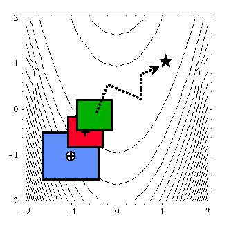
Fig. 55 SBO iteration progression for model hierarchies.
When applying corrections to the low-fidelity model, there is no concern for balancing global accuracy with the local consistency requirements. However, with only a single high-fidelity model evaluation at the center of each trust region, it is critical to use the best correction possible on the low-fidelity model in order to achieve rapid convergence rates to the optimum of the high-fidelity model [EGC04].
A multifidelity test problem named dakota_sbo_hierarchical.in
is available in dakota/share/dakota/test to demonstrate this
SBO approach. This test problem uses the Rosenbrock function as the high
fidelity model and a function named “lf_rosenbrock” as the low fidelity
model. Here, lf_rosenbrock is a variant of the Rosenbrock function
(see dakota_source/test/lf_rosenbrock.C
for formulation) with the minimum point at
\((x_1,x_2)=(0.80,0.44)\), whereas the minimum of the original
Rosenbrock function is \((x_1,x_2)=(1,1)\). Multifidelity SBO
locates the high-fidelity minimum in 11 high fidelity evaluations for
additive second-order corrections and in 208 high fidelity evaluations
for additive first-order corrections, but fails for zeroth-order
additive corrections by converging to the low-fidelity minimum.
SBO with Reduced Order Models
When performing SBO with reduced-order models (ROMs), the ROM is mathematically generated from the high-fidelity model. A critical issue in this ROM generation is the ability to capture the effect of parametric changes within the ROM. Two approaches to parametric ROM are extended ROM (E-ROM) and spanning ROM (S-ROM) techniques [WEM06]. Closely related techniques include tensor singular value decomposition (SVD) methods [LMV00]. In the single-point and multipoint E-ROM cases, the SBO iteration can appear as in Fig. 55, whereas in the S-ROM, global E-ROM, and tensor SVD cases, the SBO iteration will appear as in Fig. 54. In addition to the high-fidelity model analysis requirements, procedures for updating the system matrices and basis vectors are also required.
Relative to data fits and multifidelity models, ROMs have some attractive advantages. Compared to data fits such as regression-based polynomial models, they are more physics-based and would be expected to be more predictive (e.g., in extrapolating away from the immediate data). Compared to multifidelity models, ROMS may be more practical in that they do not require multiple computational models or meshes which are not always available. The primary disadvantage is potential invasiveness to the simulation code for projecting the system using the reduced basis.
Surrogate-Based Global Minimization
In surrogate-based global minimization, the optimization method operates over the whole domain on a global surrogate constructed over a (static or adaptively augmented) set of truth model sample points. There are no trust regions and no convergence guarantees for the original optimization problem, though optimizers can be reasonably expected to converge as expected on the approximate (surrogate) problem.
In the first, and perhaps most common, global surrogate use case, a user wishes to use existing function evaluations or a fixed sample size (perhaps based on computational cost and allocation of resources) to build a surrogate once and optimize on it. For this single global optimization on a surrogate model, the set of surrogate build points is determined in advance. Contrast this with trust-region local methods in which the number of “true” function evaluations depends on the location and size of the trust region, the goodness of the surrogate within it, and overall problem characteristics. Any Dakota optimizer can be used with a (build-once) global surrogate by specifying the of a global surrogate model with the optimizer’s keyword.
The more tailored, adaptive method supports the second use case: globally updating the surrogate during optimization. This method iteratively adds points to the sample set used to create the surrogate, rebuilds the surrogate, and then performs global optimization on the new surrogate. Thus, surrogate-based global optimization can be used in an iterative scheme. In one iteration, minimizers of the surrogate model are found, and a selected subset of these are passed to the next iteration. In the next iteration, these surrogate points are evaluated with the “truth” model, and then added to the set of points upon which the next surrogate is constructed. This presents a more accurate surrogate to the minimizer at each subsequent iteration, presumably driving to optimality quickly. Note that a global surrogate is constructed using the same bounds in each iteration. This approach has no guarantee of convergence.
The surrogate-based global method was originally designed for MOGA (a multi-objective genetic algorithm). Since genetic algorithms often need thousands or tens of thousands of points to produce optimal or near-optimal solutions, surrogates can help by reducing the necessary truth model evaluations. Instead of creating one set of surrogates for the individual objectives and running the optimization algorithm on the surrogate once, the idea is to select points along the (surrogate) Pareto frontier, which can be used to supplement the existing points. In this way, one does not need to use many points initially to get a very accurate surrogate. The surrogate becomes more accurate as the iterations progress.
Most single objective optimization methods will return only a single
optimal point. In that case, only one point from the surrogate model
will be evaluated with the “true” function and added to the pointset
upon which the surrogate is based. In this case, it will take many
iterations of the surrogate-based global optimization for the approach
to converge, and its utility may not be as great as for the
multi-objective case when multiple optimal solutions are passed from one
iteration to the next to supplement the surrogate. Note that the user
has the option of appending the optimal points from the surrogate model
to the current set of truth points or using the optimal points from the
surrogate model to replace the optimal set of points from the previous
iteration. Although appending to the set is the default behavior, at
this time we strongly recommend using the option replace_points
because it appears to be more accurate and robust.
When using the surrogate-based global method, we first recommend running
one optimization on a single surrogate model. That is, set
max_iterations to 1. This will allow one to get a sense of where the
optima are located and also what surrogate types are the most accurate
to use for the problem. Note that by fixing the seed of the sample on
which the surrogate is built, one can take a Dakota input file, change
the surrogate type, and re-run the problem without any additional
function evaluations by specifying the use of the dakota restart file
which will pick up the existing function evaluations, create the new
surrogate type, and run the optimization on that new surrogate. Also
note that one can specify that surrogates be built for all primary
functions and constraints or for only a subset of these functions and
constraints. This allows one to use a “truth” model directly for some of
the response functions, perhaps due to them being much less expensive
than other functions. Finally, a diagnostic threshold can be used to
stop the method if the surrogate is so poor that it is unlikely to
provide useful points. If the goodness-of-fit has an R-squared value
less than 0.5, meaning that less than half the variance of the output
can be explained or accounted for by the surrogate model, the
surrogate-based global optimization stops and outputs an error message.
This is an arbitrary threshold, but generally one would want to have an
R-squared value as close to 1.0 as possible, and an R-squared value
below 0.5 indicates a very poor fit.
For the surrogate-based global method, we initially recommend a small number of maximum iterations, such as 3–5, to get a sense of how the optimization is evolving as the surrogate gets updated globally. If it appears to be changing significantly, then a larger number (used in combination with restart) may be needed.
Listing 61 shows a Dakota input file
that implements surrogate-based global optimization on a multi-objective
test function. The first method keyword block contains the keyword
surrogate_based_global, plus the commands for specifying five as the
maximum iterations and the option to replace points in the global
surrogate construction. The method block identified as MOGA specifies a
multi-objective genetic algorithm optimizer and its controls. The model
keyword block specifies a surrogate model. In this case, a
gaussian_process model is used as a surrogate. The
dace_method_pointer specifies that the surrogate will be build on
100 Latin Hypercube samples with a seed = 531. The remainder of the
input specification deals with the interface to the actual analysis
driver and the 2 responses being returned as objective functions from
that driver.
# Dakota Input File: mogatest1_opt_sbo.in

environment
  tabular_data
    tabular_data_file = 'mogatest1_opt_sbo.dat'
  top_method_pointer = 'SBGO'

method
  id_method = 'SBGO'
  surrogate_based_global
    model_pointer = 'SURROGATE'
    method_pointer = 'MOGA'
    max_iterations = 5
    replace_points
  output verbose

method
  id_method = 'MOGA'
  moga
        seed = 10983
    population_size = 300
    max_function_evaluations = 5000
    initialization_type unique_random
    crossover_type shuffle_random
        num_offspring = 2 num_parents = 2
        crossover_rate = 0.8
    mutation_type replace_uniform
        mutation_rate = 0.1
    fitness_type domination_count
    replacement_type below_limit = 6
        shrinkage_percentage = 0.9
    niching_type distance 0.05 0.05
    postprocessor_type
        orthogonal_distance 0.05 0.05
    convergence_type metric_tracker
        percent_change = 0.05 num_generations = 10
  output silent

model
    id_model = 'SURROGATE'
    surrogate global
        dace_method_pointer = 'SAMPLING'
        correction additive zeroth_order
        gaussian_process dakota

method
    id_method = 'SAMPLING'
    sampling
      samples = 100
      seed = 531
      sample_type lhs
      model_pointer = 'TRUTH'

model
    id_model = 'TRUTH'
    single
      interface_pointer = 'TRUE_FN'

variables
    continuous_design = 3
        initial_point      0     0     0
        upper_bounds       4     4     4
        lower_bounds      -4    -4    -4
        descriptors      'x1'  'x2'  'x3'

interface
    id_interface = 'TRUE_FN'
    analysis_drivers = 'mogatest1'
      direct

responses
    objective_functions = 2
    no_gradients
    no_hessians
Footnotes
- footnote_hybridfit
It is also possible to use a hybrid data fit/multifidelity approach in which a smooth data fit of a noisy low fidelity model is used in combination with a high fidelity model