Optimization
Optimization algorithms work to minimize (or maximize) an objective function, typically calculated by the user simulation code, subject to constraints on design variables and responses. Available approaches in Dakota include well-tested and proven gradient-based, derivative-free local, and global methods for use in science and engineering design applications. Dakota also offers more advanced algorithms, e.g., to manage multi-objective optimization or perform surrogate-based minimization. This page summarizes optimization problem formulation, standard algorithms available in Dakota (mostly through included third party libraries), some advanced capabilities, and offers usage guidelines.
Optimization Formulations
This section provides a basic introduction to the mathematical formulation of optimization problems. The primary goal of this section is to introduce terms relating to these topics and is not intended to be a description of theory or numerical algorithms. For further details, consult [Aro89], [GMW81], [HG92], [NJ99], and [Van84].
A general optimization problem is formulated as follows:
where vector and matrix terms are marked in bold typeface. In this formulation, \(\mathbf{x}=[x_{1},x_{2},\ldots,x_{n}]\) is an n-dimensional vector of real-valued design variables or design parameters. The n-dimensional vectors, \(\mathbf{x}_{L}\) and \(\mathbf{x}_U\), are the lower and upper bounds, respectively, on the design parameters. These bounds define the allowable values for the elements of \(\mathbf{x}\), and the set of all allowable values is termed the design space or the parameter space. A design point or a sample point is a particular set of values within the parameter space.
The optimization goal is to minimize the objective function, \(f(\mathbf{x})\), while satisfying the constraints. Constraints can be categorized as either linear or nonlinear and as either inequality or equality. The nonlinear inequality constraints, \(\mathbf{g(x)}\), are “2-sided,” in that they have both lower and upper bounds, \(\mathbf{g}_L\) and \(\mathbf{g}_U\), respectively. The nonlinear equality constraints, \(\mathbf{h(x)}\), have target values specified by \(\mathbf{h}_{t}\). The linear inequality constraints create a linear system \(\mathbf{A}_i\mathbf{x}\), where \(\mathbf{A}_i\) is the coefficient matrix for the linear system. These constraints are also 2-sided as they have lower and upper bounds, \(\mathbf{a}_L\) and \(\mathbf{a}_U\), respectively. The linear equality constraints create a linear system \(\mathbf{A}_e\mathbf{x}\), where \(\mathbf{A}_e\) is the coefficient matrix for the linear system and \(\mathbf{a}_{t}\) are the target values. The constraints partition the parameter space into feasible and infeasible regions. A design point is said to be feasible if and only if it satisfies all of the constraints. Correspondingly, a design point is said to be infeasible if it violates one or more of the constraints.
Many different methods exist to solve the optimization problem given by Equation (35), all of which iterate on \(\mathbf{x}\) in some manner. That is, an initial value for each parameter in \(\mathbf{x}\) is chosen, the response quantities, \(f(\mathbf{x})\), \(\mathbf{g(x)}\), \(\mathbf{h(x)}\), are computed, often by running a simulation, and some algorithm is applied to generate a new \(\mathbf{x}\) that will either reduce the objective function, reduce the amount of infeasibility, or both. To facilitate a general presentation of these methods, three criteria will be used in the following discussion to differentiate them: optimization problem type, search goal, and search method.
Problem Classification
The optimization problem type can be characterized both by the types of constraints present in the problem and by the linearity or nonlinearity of the objective and constraint functions. For constraint categorization, a hierarchy of complexity exists for optimization algorithms, ranging from simple bound constraints, through linear constraints, to full nonlinear constraints. By the nature of this increasing complexity, optimization problem categorizations are inclusive of all constraint types up to a particular level of complexity. That is, an unconstrained problem has no constraints, a bound-constrained problem has only lower and upper bounds on the design parameters, a linearly-constrained problem has both linear and bound constraints, and a nonlinearly-constrained problem may contain the full range of nonlinear, linear, and bound constraints. If all of the linear and nonlinear constraints are equality constraints, then this is referred to as an equality-constrained problem, and if all of the linear and nonlinear constraints are inequality constraints, then this is referred to as an inequality-constrained problem. Further categorizations can be made based on the linearity of the objective and constraint functions. A problem where the objective function and all constraints are linear is called a linear programming (LP) problem. These types of problems commonly arise in scheduling, logistics, and resource allocation applications. Likewise, a problem where at least some of the objective and constraint functions are nonlinear is called a nonlinear programming (NLP) problem. These NLP problems predominate in engineering applications and are the primary focus of Dakota.
The search goal refers to the ultimate objective of the optimization algorithm, i.e., either global or local optimization. In global optimization, the goal is to find the design point that gives the lowest feasible objective function value over the entire parameter space. In contrast, in local optimization, the goal is to find a design point that is lowest relative to a “nearby” region of the parameter space. In almost all cases, global optimization will be more computationally expensive than local optimization. Thus, the user must choose an optimization algorithm with an appropriate search scope that best fits the problem goals and the computational budget.
The search method refers to the approach taken in the optimization algorithm to locate a new design point that has a lower objective function or is more feasible than the current design point. The search method can be classified as either gradient-based or nongradient-based. In a gradient-based algorithm, gradients of the response functions are computed to find the direction of improvement. Gradient-based optimization is the search method that underlies many efficient local optimization methods. However, a drawback to this approach is that gradients can be computationally expensive, inaccurate, or even nonexistent. In such situations, nongradient-based search methods may be useful. There are numerous approaches to nongradient-based optimization. Some of the more well known of these include pattern search methods (nongradient-based local techniques) and genetic algorithms (nongradient-based global techniques).
Because of the computational cost of running simulation models, surrogate-based optimization (SBO) methods are often used to reduce the number of actual simulation runs. In SBO, a surrogate or approximate model is constructed based on a limited number of simulation runs. The optimization is then performed on the surrogate model. Dakota has an extensive framework for managing a variety of local, multipoint, global, and hierarchical surrogates for use in optimization. Finally, sometimes there are multiple objectives that one may want to optimize simultaneously instead of a single scalar objective. In this case, one may employ multi-objective methods that are described below.
This overview of optimization approaches underscores that no single optimization method or algorithm works best for all types of optimization problems. The Optimization Usage Guidelines section offers guidelines for choosing a Dakota optimization algorithm best matched to your specific optimization problem.
Constraint Considerations
Dakota’s input commands permit the user to specify two-sided nonlinear
inequality constraints of the form
\(g_{L_{i}} \leq g_{i}(\mathbf{x})
\leq g_{U_{i}}\), as well as nonlinear equality constraints of the form
\(h_{j}(\mathbf{x}) = h_{t_{j}}\). Some optimizers (e.g.,
those in the NPSOL and OPTPP family, soga,
and moga methods) can handle these
constraint forms directly, whereas other optimizers (e.g.,
asynch_pattern_search, mesh_adaptive_search,
those in the DOT and CONMIN families) require Dakota to perform an internal
conversion of all constraints to one-sided inequality constraints of the
form \(g_{i}(\mathbf{x}) \leq 0\). In the latter case, the two-sided
inequality constraints are treated as
\(g_{i}(\mathbf{x}) - g_{U_{i}} \leq 0\) and \(g_{L_{i}} -
g_{i}(\mathbf{x}) \leq 0\) and the equality constraints are treated as
\(h_{j}(\mathbf{x}) - h_{t_{j}} \leq 0\) and \(h_{t_{j}} -
h_{j}(\mathbf{x}) \leq 0\).
The situation is similar for linear constraints: asynch_pattern_search,
soga, moga, NPSOL, and OPTPP methods support them
directory, whereas DOT and CONMIN methods do not.
For linear inequalities of the form \(a_{L_{i}} \leq \mathbf{a}_{i}^{T}\mathbf{x} \leq a_{U_{i}}\) and linear equalities of the form \(\mathbf{a}_{i}^{T}\mathbf{x} = a_{t_{j}}\), the nonlinear constraint arrays in DOT and CONMIN methods are further augmented to include \(\mathbf{a}_{i}^{T}\mathbf{x} - a_{U_{i}} \leq 0\) and \(a_{L_{i}} - \mathbf{a}_{i}^{T}\mathbf{x} \leq 0\) in the inequality case and \(\mathbf{a}_{i}^{T}\mathbf{x} - a_{t_{j}} \leq 0\) and \(a_{t_{j}} - \mathbf{a}_{i}^{T}\mathbf{x} \leq 0\) in the equality case. Awareness of these constraint augmentation procedures can be important for understanding the diagnostic data returned from the DOT and CONMIN methods.
Other optimizers fall somewhere in between. NLPQL methods support nonlinear
equality constraints \(h_{j}(\mathbf{x}) = 0\) and nonlinear one-sided inequalities
\(g_{i}(\mathbf{x}) \geq 0\), but does not natively support linear
constraints. Constraint mappings are used with NLPQL for both linear and
nonlinear cases. Most COLINY methods now support two-sided
nonlinear inequality constraints and nonlinear constraints with targets,
but do not natively support linear constraints. ROL’s (rol)
augmented Lagrangian method converts inequality constraints into
equality constraints with bounded slack variables. This conversion is
performed internally within ROL, but might explain potentially weak
convergence rates for problems with large number of inequality
constraints.
When gradient and Hessian information is used in the optimization, derivative components are most commonly computed with respect to the active continuous variables, which in this case are the continuous design variables. This differs from parameter study methods (for which all continuous variables are active) and from non-deterministic analysis methods (for which the uncertain variables are active). Refer to the Active Variables for Derivatives section for additional information on derivative components and active continuous variables.
Optimizing with Dakota: Choosing a Method
This section summarizes the optimization methods available in Dakota. We group them according to search method and search goal and establish their relevance to types of problems. For a summary of this discussion, see Optimization Usage Guidelines.
Gradient-Based Local Methods
Gradient-based optimizers are best suited for efficient navigation to a local minimum in the vicinity of the initial point. They are not intended to find global optima in nonconvex design spaces. For global optimization methods, see Derivative-Free Global Methods. Gradient-based optimization methods are highly efficient, with the best convergence rates of all of the local optimization methods, and are the methods of choice when the problem is smooth, unimodal, and well-behaved. However, these methods can be among the least robust when a problem exhibits nonsmooth, discontinuous, or multimodal behavior. The derivative-free methods described in Derivative-Free Local Methods are more appropriate for problems with these characteristics.
Gradient accuracy is a critical factor for gradient-based optimizers, as inaccurate derivatives will often lead to failures in the search or premature termination of the method. Analytic gradients and Hessians are ideal but often unavailable. If analytic gradient and Hessian information can be provided by an application code, a full Newton method will achieve quadratic convergence rates near the solution. If only gradient information is available and the Hessian information is approximated from an accumulation of gradient data, superlinear convergence rates can be obtained. It is most often the case for engineering applications, however, that a finite difference method will be used by the optimization algorithm to estimate gradient values. Dakota allows the user to select the step size for these calculations, as well as choose between forward-difference and central-difference algorithms. The finite difference step size should be selected as small as possible, to allow for local accuracy and convergence, but not so small that the steps are “in the noise.” This requires an assessment of the local smoothness of the response functions using, for example, a parameter study method. Central differencing will generally produce more reliable gradients than forward differencing but at roughly twice the expense.
Gradient-based methods for nonlinear optimization problems can be described as iterative processes in which a sequence of subproblems, usually which involve an approximation to the full nonlinear problem, are solved until the solution converges to a local optimum of the full problem. The optimization methods available in Dakota fall into several categories, each of which is characterized by the nature of the subproblems solved at each iteration.
Methods for Unconstrained Problems
For unconstrained problems, conjugate gradient methods can be applied
which require first derivative information. The subproblems entail
minimizing a quadratic function over a space defined by the gradient and
directions that are mutually conjugate with respect to the Hessian.
There are a couple of options in terms of methods to be used strictly
for unconstrained problems, namely the Polak-Ribiere conjugate gradient
method (optpp_cg) and ROL’s (Rapid Optimization Library for
large-scale optimization, part of the Trilinos software
suite [KRvBWvW14]) trust-region method with truncated
conjugate gradient subproblem solver (rol). ROL relies on secant
updates for the Hessian, with the approximation to the Hessian matrix
at each iteration provided using only values of the gradient at current
and previous iterates.
Note that ROL has been developed for, and mostly applied to, problems with analytic gradients/Hessians. Nonetheless, ROL can be used with Dakota-, or vendor-provided finite-differencing approximations to the gradient of the objective function. However, a user relying on such approximations is advised to use alternative optimizers that exhibit better performance in those scenarios.
Methods for Bound-Constrained Problems
For bound-constrained problems, both conjugate gradient methods and
quasi-Newton methods (described in the next sub-section) are available
in Dakota. For conjugate gradient methods, the Fletcher-Reeves conjugate
gradient method (conmin_frcg and
dot_frcg [Vanderplaats Research and Development, Inc.95]) and ROL’s trust-region method
with truncated conjugate gradient subproblem solver (rol) are
available. Note that ROL exhibits slow/erratic convergence when
finite-differencing approximations to the gradient of objective function
are used. DOT (dot_bfgs) provides a quasi-Newton method for such
problems.
Warning
In DOT version 4.20, we have noticed inconsistent behavior of dot_frcg
across different versions of Linux. Our best assessment is that it is
due to different treatments of uninitialized variables. As we do not
know the intention of the code authors and maintaining DOT source code
is outside of the Dakota project scope, we have not made nor are we
recommending any code changes to address this. However, all users who
use dot_frcg in DOT 4.20 should be aware that results may
not be reliable.
Methods for Constrained Problems
For constrained problems, the available methods fall under one of four categories, namely Sequential Quadratic Programming (SQP) methods, Newton methods, Method of Feasible Directions (MFD) methods, and the augmented Lagrangian method.
Sequential Quadratic Programming (SQP) methods are appropriate for nonlinear optimization problems with nonlinear constraints. Each subproblem involves minimizing a quadratic approximation of the Lagrangian subject to linearized constraints. Only gradient information is required; Hessians are approximated by low-rank updates defined by the step taken at each iterations.
Warning
While the solution found by an SQP method will respect the constraints, the intermediate iterates may not. Dakota optimization methods that respect lienar constraints throughout
SQP methods available in Dakota include
dot_sqp, nlpql_sqp, and npsol_sqp
[GMSW86]. The particular implementation in nlpql_sqp [Sch04]
uses a variant with distributed and non-monotonic line search. Thus, this
variant is designed to be more robust in the presence of inaccurate or
noisy gradients common in many engineering applications. ROL’s
composite-step method (rol), utilizing SQP with trust regions,
for equality-constrained problems is another option (Note that ROL exhibits
slow/erratic convergence when finite-differencing approximations to the
gradient of objective and constraints are used). Also available is a
method related to SQP: sequential linear programming (dot_slp).
Newton Methods can be applied to nonlinear optimization problems with
nonlinear constraints. The subproblems associated with these methods
entail finding the solution to a linear system of equations derived by
setting the derivative of a second-order Taylor series expansion to
zero. Unlike SQP methods, Newton methods maintain feasibility over the
course of the optimization iterations. The variants of this approach
correspond to the amount of derivative information provided by the user.
The full Newton method (optpp_newton) expects both gradients and
Hessians to be provided. Quasi-Newton methods (optpp_q_newton)
expect only gradients. The Hessian is approximated by the
Broyden-Fletcher-Goldfarb-Shanno (BFGS) low-rank updates. Finally, the
finite difference Newton method (optpp_fd_newton) expects only
gradients and approximates the Hessian with second-order finite
differences.
Method of Feasible Directions (MFD) methods are appropriate for
nonlinear optimization problems with nonlinear constraints. These
methods ensure that all iterates remain feasible. Dakota includes
conmin_mfd [Van73] and dot_mmfd
Note
One observed drawback to conmin_mfd is that it does a poor job
handling equality constraints. dot_mmfd does not suffer from this
problem, nor do other methods for constrained problems.
The augmented Lagrangian method provides a strategy to handle equality
and inequality constraints by introducing the augmented Lagrangian
function, combining the use of Lagrange multipliers and a quadratic
penalty term. It is implemented in ROL (rol) exhibiting scalable
performance for large-scale problems. As previously stated, ROL exhibits
slow/erratic convergence when finite-differencing approximations to the
gradient of objective function and/or constraints are used. Users are
advised to resort to alternative optimizers until performance of ROL
improves in future releases.
Warning
Not all Dakota methods strictly respect linear constraints. Those that
propose only feasible candidate design points include asynch_pattern_search,
npsol_sqp, and the OPTPP family of methods, with the exception of
optpp_fd_newton. Other methods seek feasible solutions, but may
violate linear constraints as they run.
Derivative-Free Local Methods
Derivative-free methods can be more robust and more inherently parallel than gradient-based approaches. They can be applied in situations were gradient calculations are too expensive or unreliable. In addition, some derivative-free methods can be used for global optimization, while gradient-based techniques, by themselves, cannot. For these reasons, derivative-free methods are often go-to methods when the problem may be nonsmooth, multimodal, or poorly behaved. It is important to be aware, however, that they exhibit much slower convergence rates for finding an optimum, and as a result, tend to be much more computationally demanding than gradient-based methods. They often require from several hundred to a thousand or more function evaluations for local methods, depending on the number of variables, and may require from thousands to tens-of-thousands of function evaluations for global methods. Given the computational cost, it is often prudent to use derivative-free methods to identify regions of interest and then use gradient-based methods to home in on the solution. In addition to slow convergence, nonlinear constraint support in derivative-free methods is an open area of research and, while supported by many methods in Dakota, is not as refined as constraint support in gradient-based methods.
Method Descriptions
Pattern Search methods can be applied to nonlinear optimization
problems with nonlinear constraints. They generally walk through the domain
according to a defined stencil of search directions. These methods are
best suited for efficient navigation to a local minimum in the vicinity
of the initial point; however, they sometimes exhibit limited global
identification abilities if the stencil is such that it allows them to
step over local minima. There are two main pattern search methods
available in Dakota, and they vary according to richness of available
stencil and the way constraints are supported. Asynchronous Parallel Pattern
Search (APPS) [GK06] (asynch_pattern_search)
uses the coordinate basis as its stencil, and it handles nonlinear
constraints explicitly through modification of the coordinate stencil to
allow directions that parallel constraints [GK07]. A
second variant of pattern search, coliny_pattern_search, has the
option of using either a coordinate or a simplex basis as well as
allowing more options for the stencil to evolve over the course of the
optimization. It handles nonlinear constraints through the use of
penalty functions.
The mesh_adaptive_search [ALeDigabelT09], [AAC+], [LeDigabel11]
is similar in spirit to and falls in the same class of methods as the
pattern search methods. The primary difference is that its underlying
search structure is that of a mesh. The mesh_adaptive_search also
provides a unique optimization capability in Dakota in that it can
explicitly treat categorical variables, i.e., non-relaxable discrete
variables. Furthermore,
it provides the ability to use a surrogate model to inform the priority
of function evaluations with the goal of reducing the number needed.
Simplex methods for nonlinear optimization problem are similar to
pattern search methods, but their search directions are defined by
triangles that are reflected, expanded, and contracted across the
variable space. The two simplex-based methods available in Dakota are
the Parallel Direct Search method [DT94]
(optpp_pds) and the Constrained Optimization BY Linear
Approximations (COBYLA) (coliny_cobyla). The former handles only
bound constraints, while the latter handles nonlinear constraints.
Note
One drawback of both simplex-based methods is that their current implementations do not allow them to take advantage of parallel computing resources via Dakota’s infrastructure. Additionally, we note that the implementation of COBYLA is such that the best function value is not always returned to Dakota for reporting. The user is advised to look through the Dakota screen output or the tabular output file (if generated) to confirm what the best function value and corresponding parameter values are. Furthermore, COBYLA does not always respect bound constraints when scaling is turned on. Neither bug will be fixed, as maintaining third-party source code (such as COBYLA) is outside of the Dakota project scope.
A Greedy Search Heuristic for nonlinear optimization problems is
captured in the Solis-Wets (coliny_solis_wets) method.
This method takes a sampling-based approach in order to identify search directions.
Note
An observed drawback to coliny_solis_wets is that it does a
poor job solving problems with nonlinear constraints. This algorithm is also
not implemented in such a way as to
take advantage of parallel computing resources via Dakota’s
infrastructure.
Nonlinear Optimization with Path Augmented Constraints (NOWPAC) is a
provably-convergent gradient-free inequality-constrained optimization
method that solves a series of trust region surrogate-based subproblems
to generate improving steps. Due to its use of an interior penalty
scheme and enforcement of strict feasibility,
nowpac [AM14] does not support
linear or nonlinear equality constraints. The stochastic version is
snowpac, which incorporates noise estimates in its objective and
inequality constraints. snowpac modifies its trust region controls
and adds smoothing from a Gaussian process surrogate in order to
mitigate noise.
Note
Unlike the stochastic version (snowpac), nowpac does
not currently support a feasibility restoration mode, so it is necessary to start from
a feasible design. Also, (s)nowpac is not configured with Dakota by default
and requires a separate installation of the NOWPAC distribution, along
with third-party libraries Eigen and NLOPT.
Example
The Dakota input file shown in Listing 47 applies a pattern search method to minimize the Rosenbrock function. We note that this example is used as a means of demonstrating the contrast between input files for gradient-based and derivative-free optimization. Since derivatives can be computed analytically and efficiently, the preferred approach to solving this problem is a gradient-based method.
The Dakota input file shown in
Listing 47
is similar to the input file for the gradient-based optimization, except
it has a different set of keywords in the method block,, and the gradient
specification in the responses block has been
changed to no_gradients. The pattern search optimization algorithm
used, coliny_pattern_search is part of the SCOLIB
library [Har07]. See the Keyword Reference
for more information on the method
block commands that can be used with SCOLIB algorithms.
dakota/share/dakota/examples/users/rosen_opt_patternsearch.in# Dakota Input File: rosen_opt_patternsearch.in
environment
tabular_data
tabular_data_file = 'rosen_opt_patternsearch.dat'
method
coliny_pattern_search
initial_delta = 0.5
solution_target = 1e-4
exploratory_moves
basic_pattern
contraction_factor = 0.75
max_iterations = 1000
max_function_evaluations = 2000
variable_tolerance = 1e-4
model
single
variables
continuous_design = 2
initial_point 0.0 0.0
lower_bounds -2.0 -2.0
upper_bounds 2.0 2.0
descriptors 'x1' "x2"
interface
analysis_drivers = 'rosenbrock'
direct
responses
objective_functions = 1
no_gradients
no_hessians
For this run, the optimizer was given an initial design point of \((x_1,x_2) = (0.0,0.0)\) and was limited to 2000 function evaluations. In this case, the pattern search algorithm stopped short of the optimum at \((x_1,x_2) = (1.0,1,0)\), although it was making progress in that direction when it was terminated. (It would have reached the minimum point eventually.)
Fig. 46 shows the locations of the function evaluations used in the pattern search algorithm. Fig. 47 provides a close-up view of the pattern search function evaluations used at the start of the algorithm. The coordinate pattern is clearly visible at the start of the iteration history, and the decreasing size of the coordinate pattern is evident at the design points move toward \((x_1,x_2) = (1.0,1.0)\).
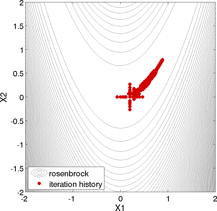
Fig. 46 Rosenbrock pattern search: sequence of design points (dots) evaluated
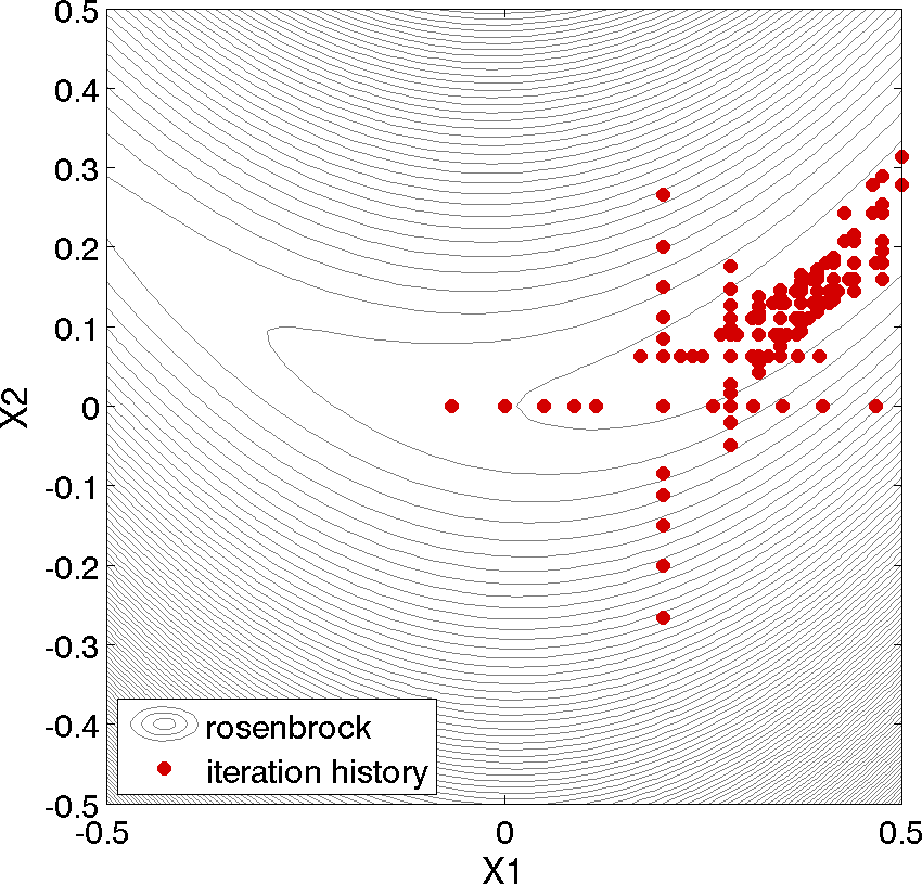
Fig. 47 Rosenbrock pattern search: close-up view illustrating the shape of the coordinate pattern used
While pattern search algorithms are useful in many optimization problems, this example shows some of the drawbacks to this algorithm. While a pattern search method may make good initial progress towards an optimum, it is often slow to converge. On a smooth, differentiable function such as Rosenbrock’s function, a nongradient-based method will not be as efficient as a gradient-based method. However, there are many engineering design applications where gradient information is inaccurate or unavailable, which renders gradient-based optimizers ineffective. Thus, pattern search algorithms are often good choices in complex engineering applications when the quality of gradient data is suspect.
Derivative-Free Global Methods
Much of the discussion of Derivative-Free Local Methods is also applicable to derivative-free global methods, so we forego repeating it here. There are two types of global optimization methods in Dakota.
Method Descriptions
Evolutionary Algorithms (EA) are based on Darwin’s theory of
survival of the fittest. The EA algorithm starts with a randomly
selected population of design points in the parameter space, where the
values of the design parameters form a “genetic string,” analogous to
DNA in a biological system, that uniquely represents each design point
in the population. The EA then follows a sequence of generations, where
the best design points in the population (i.e., those having low
objective function values) are considered to be the most “fit” and are
allowed to survive and reproduce. The EA simulates the evolutionary
process by employing the mathematical analogs of processes such as
natural selection, breeding, and mutation. Ultimately, the EA identifies
a design point (or a family of design points) that minimizes the
objective function of the optimization problem. An extensive discussion
of EAs is beyond the scope of this text, but may be found in a variety
of sources (cf., [HG92] pp.
149-158; [Gol89]). EAs available in Dakota include
coliny_ea, soga, and moga.
The latter is specifically designed for multi-objective problems, discussed further
below. All variants can optimize over discrete
variables, including discrete string variables, in addition to
continuous variables.
DIvision of RECTangles (DIRECT) [Gab01] balances
local search in promising regions of the design space with global search
in unexplored regions. It adaptively subdivides the space of feasible
design points to guarantee that iterates are generated in the
neighborhood of a global minimum in finitely many iterations. Dakota
includes two implementations (ncsu_direct and
coliny_direct). In practice, DIRECT has proven an effective
heuristic for many applications. For some problems, the ncsu_direct
implementation has outperformed the coliny_direct implementation.
ncsu_direct can accommodate only bound constraints, while
coliny_direct handles nonlinear constraints using a penalty
formulation of the problem.
Efficient Global Optimization (EGO) is a global optimization
technique that employs response surface
surrogates [HANZ06, JSW98]. The efficient_global
method is Dakota’s implementation of EGO.
In each EGO iteration, a Gaussian process (GP) approximation for the objective function is constructed based on sample points of the true simulation. The GP allows one to specify the prediction at a new input location as well as the uncertainty associated with that prediction. The key idea in EGO is to maximize an Expected Improvement Function (EIF), defined as the expectation that any point in the search space will provide a better solution than the current best solution, based on the expected values and variances predicted by the GP model.
It is important to understand how the use of this EIF leads to optimal solutions. The EIF indicates how much the objective function value at a new potential location is expected to be less than the predicted value at the current best solution. Because the GP model provides a Gaussian distribution at each predicted point, expectations can be calculated. Points with good expected values and even a small variance will have a significant expectation of producing a better solution (exploitation), but so will points that have relatively poor expected values and greater variance (exploration). The EIF incorporates both the idea of choosing points which minimize the objective and choosing points about which there is large prediction uncertainty (e.g., there are few or no samples in that area of the space, and thus the probability may be high that a sample value is potentially lower than other values). Because the uncertainty is higher in regions of the design space with few observations, this provides a balance between exploiting areas of the design space that predict good solutions, and exploring areas where more information is needed.
There are two major differences between our implementation and that of [JSW98]: we do not use a branch and bound method to find points which maximize the EIF. Rather, we use the DIRECT algorithm. Second, we allow for multiobjective optimization and nonlinear least squares including general nonlinear constraints. Constraints are handled through an augmented Lagrangian merit function approach (see Surrogate-Based Local Minimization).
Note
Dakota also has an experimental branch and bound capability that provides a gradient-based approach to solving mixed-variable global optimization problems. One key distinction is that it does not handle categorical variables (e.g., string variables). The branch and bound method is discussed further in the Mixed Integer Nonlinear Programming section.
Examples
Evolutionary algorithm: In contrast to pattern search algorithms, which are local optimization methods, evolutionary algorithms (EA) are global optimization methods. As was described above for the pattern search algorithm, the Rosenbrock function is not an ideal test problem for showcasing the capabilities of evolutionary algorithms. Rather, EAs are best suited to optimization problems that have multiple local optima, and where gradients are either too expensive to compute or are not readily available.
dakota/share/dakota/examples/users/rosen_opt_ea.in# Dakota Input File: rosen_opt_ea.in
environment
tabular_data
tabular_data_file = 'rosen_opt_ea.dat'
method
coliny_ea
max_iterations = 100
max_function_evaluations = 2000
seed = 11011011
population_size = 50
fitness_type merit_function
mutation_type offset_normal
mutation_rate 1.0
crossover_type two_point
crossover_rate 0.0
replacement_type chc = 10
model
single
variables
continuous_design = 2
lower_bounds -2.0 -2.0
upper_bounds 2.0 2.0
descriptors 'x1' "x2"
interface
analysis_drivers = 'rosenbrock'
direct
responses
objective_functions = 1
no_gradients
no_hessians
Listing 48 shows a Dakota input file that uses an EA to minimize the Rosenbrock function. For this example the EA has a population size of 50. At the start of the first generation, a random number generator is used to select 50 design points that will comprise the initial population. A specific seed value is used in this example to generate repeatable results.
A two-point crossover technique
is used to exchange genetic string values between the members of the
population during the EA breeding process. The result of the breeding
process is a population comprised of the 10 best “parent” design points
(elitist strategy) plus 40 new “child” design points. The EA
optimization process will be terminated after either 100 iterations
(generations of the EA) or 2,000 function evaluations. The EA software
available in Dakota provides the user with much flexibility in choosing
the settings used in the optimization process.
See coliny_ea and [Har07] for details
on these settings.
The EA optimization results printed at the end of this file show that
the best design point found was \((x_1,x_2) = (0.98,0.95)\). The
file ea_tabular.dat.sav
provides a listing of the design parameter values and objective
function values for all 2,000 design points evaluated during the running
of the EA. Fig. 48
shows the population of 50 randomly selected design points that comprise
the first generation of the EA, and Fig. 49
shows the final population of 50 design points, where most of the 50
points are clustered near \((x_1,x_2) = (0.98,0.95)\).
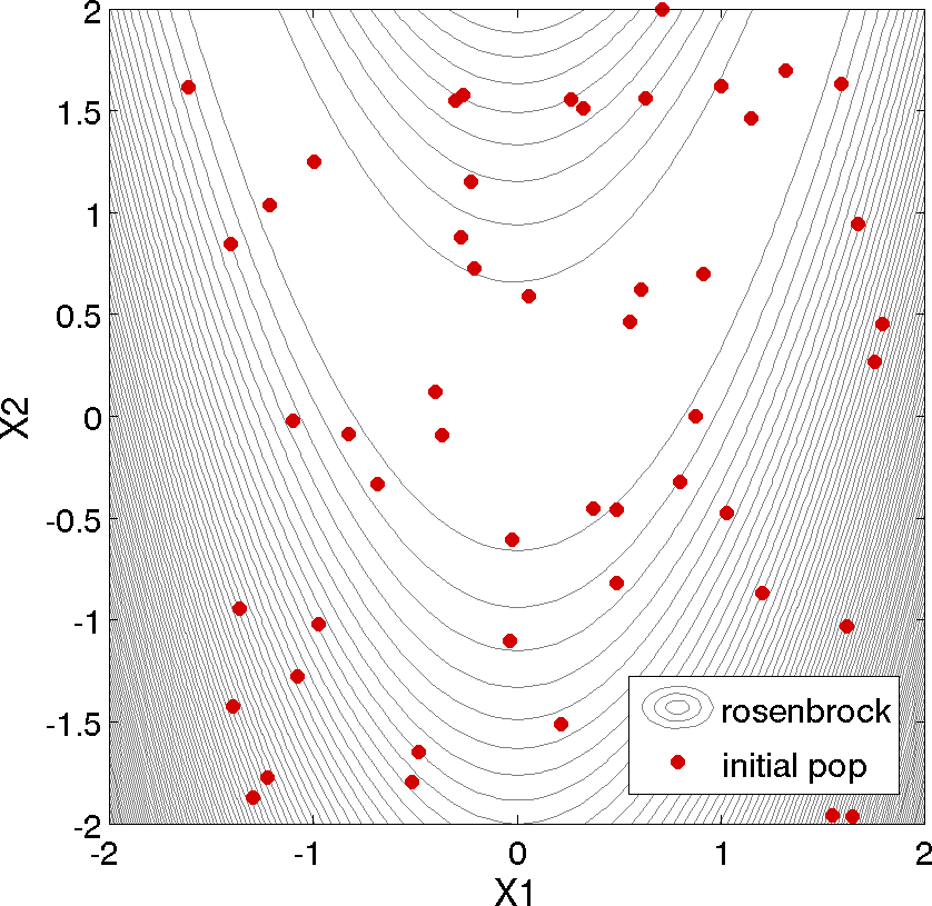
Fig. 48 50 design points in the initial population of an evolutionary algorithm
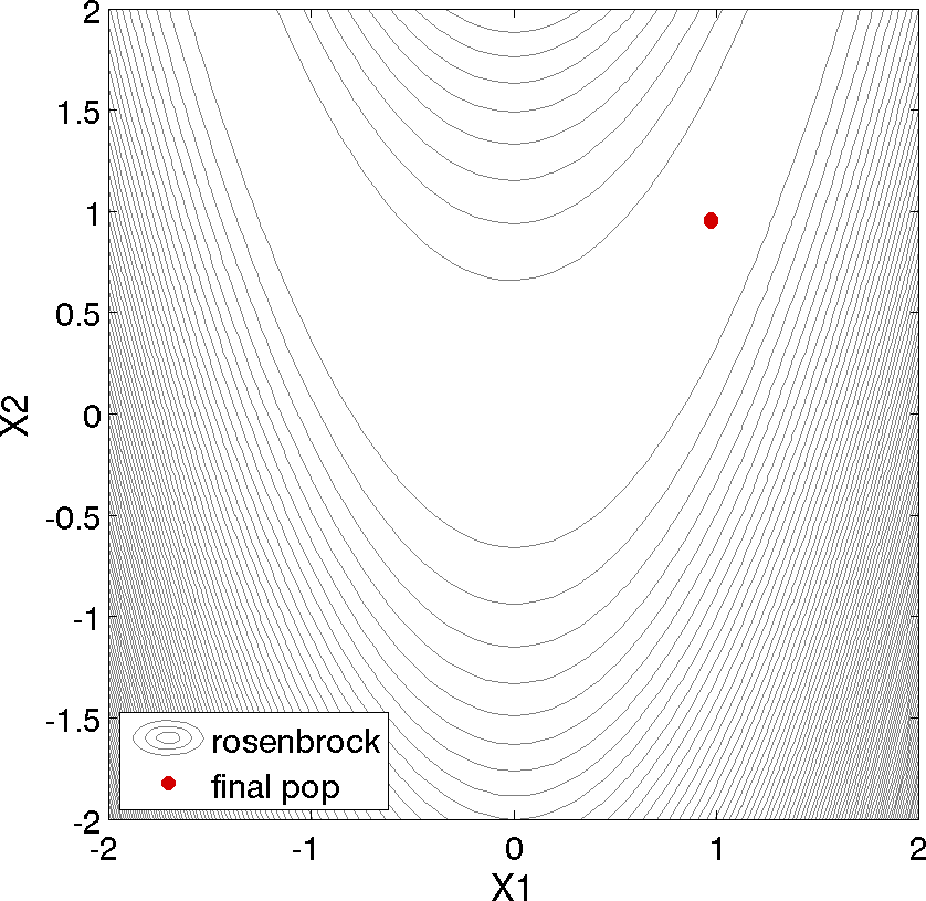
Fig. 49 The final population of design points of an evolutionary algorithm
As described above, an EA is not well-suited to an optimization problem involving a smooth, differentiable objective such as the Rosenbrock function. Rather, EAs are better suited to optimization problems where conventional gradient-based optimization fails, such as situations where there are multiple local optima and/or gradients are not available. In such cases, the computational expense of an EA is warranted since other optimization methods are not applicable or impractical.
In many optimization problems, EAs often quickly identify promising regions of the design space where the global minimum may be located. However, an EA can be slow to converge to the optimum. For this reason, it can be an effective approach to combine the global search capabilities of a EA with the efficient local search of a gradient-based algorithm in a hybrid optimization strategy. In this approach, the optimization starts by using a few iterations of a EA to provide the initial search for a good region of the parameter space (low objective function and/or feasible constraints), and then it switches to a gradient-based algorithm (using the best design point found by the EA as its starting point) to perform an efficient local search for an optimum design point. More information on this hybrid approach is provided in the Hybrid Minimization section.
Efficient Global Optimization: The method is specified as
efficient_global. Currently we do not expose any specification
controls for the underlying Gaussian process model used or for the
optimization of the expected improvement function, which is currently
performed by the NCSU DIRECT algorithm. The only item the user can
specify is a seed which is used in the Latin Hypercube Sampling to
generate the initial set of points which is used to construct the
initial Gaussian process. Parallel optimization with multiple concurrent
evaluations is possible by adjusting the batch size, which is consisted
of two smaller batches. The first batch aims at maximizing the
acquisition function, where the second batch promotes the exploration by
maximizing the variance. An example specification for the EGO algorithm
is shown in Listing 49.
dakota/share/dakota/examples/users/dakota_rosenbrock_ego.in# Dakota Input File: rosen_opt_ego.in
environment
tabular_data
tabular_data_file = 'rosen_opt_ego.dat'
method
efficient_global
seed = 123456
variables
continuous_design = 2
lower_bounds -2.0 -2.0
upper_bounds 2.0 2.0
descriptors 'x1' 'x2'
interface
analysis_drivers = 'rosenbrock'
direct
responses
objective_functions = 1
no_gradients
no_hessians
There are two types of parallelization within the efficient_global
method: the first one is batch-sequential parallel, which is active by
default, and the second one is asynchronous batch parallel. These are activated
using the blocking and
nonblocking keywords, respectively.
See dakota/share/dakota/examples/users/dakota_rosenbrock_ego_stoch.in
for how to set up an asynchronous parallel EGO study.
Both of these parallel EGO variants are enabled by setting a batch
size with the keyword batch_size.
The whole batch is further divided into two sub-batches: the
first batch focuses on querying points corresponding to maximal value
of the acquisition function, whereas the second batch focuses on
querying points with maximal posterior variances in the GP. The size
of the second batch is set with the keyword exploration,
which has to be less than or equal to batch_size - 1.
For further elaboration of the difference between batch-sequential parallel and asynchronous parallel, see the detailed discussion of Efficient Global Optimization.
Additional Optimization Capabilities
Dakota has several capabilities which extend the services provided by the optimization software packages described above. Those described in this section include:
Multiobjective optimization: There are three capabilities for multiobjective optimization in Dakota. The first is MOGA, described above. The second is the Pareto-set strategy, described in Pareto Optimization. The third is a weighting factor approach for multiobjective reduction, in which a composite objective function is constructed from a set of individual objective functions using a user-specified set of
weights. These latter two approaches work with any of the above single objective algorithms.Scaling, where any optimizer (or least squares solver described in Nonlinear Least Squares), can accept user-specified (and in some cases automatic or logarithmic) scaling of continuous design variables, objective functions (or least squares terms), and constraints. Some optimization algorithms are sensitive to the relative scaling of problem inputs and outputs, and this feature can help.
The Advanced Methods section offers details on the following component-based meta-algorithm approaches:
Sequential Hybrid Minimization: This meta-algorithm allows the user to specify a sequence of minimization methods, with the results from one method providing the starting point for the next method in the sequence. An example that is useful in many engineering design problems involves the use of a nongradient-based global optimization method (e.g., genetic algorithm) to identify promising regions of the parameter space. Solutions from these regions are provided to a gradient-based method (quasi-Newton, SQP, etc.) to perform an efficient local search for the optimum point.
Multistart Local Minimization: This meta-algorithm uses many local minimization runs (often gradient-based), each of which is started from a different initial point in the parameter space. This is an attractive approach in situations where multiple local optima are known to exist or may potentially exist in the parameter space. This approach combines the efficiency of local minimization methods with the parameter space coverage of a global stratification technique.
Pareto-Set Minimization: The Pareto-set minimization strategy allows the user to specify different sets of weights for either the individual objective functions in a multiobjective optimization problem or the individual residual terms in a least squares problem. Dakota executes each of these weighting sets as a separate minimization problem, serially or in parallel, and then outputs the set of optimal designs which define the Pareto set. Pareto set information can be useful in making trade-off decisions in engineering design problems.
Multiobjective Optimization
Multiobjective optimization refers to the simultaneous optimization of two or more objective functions. Often these are competing objectives, such as cost and performance. The optimal design in a multi-objective problem is usually not a single point. Rather, it is a set of points called the Pareto front. Each point on the Pareto front satisfies the Pareto optimality criterion, which is stated as follows: a feasible vector \(X^{*}\) is Pareto optimal if there exists no other feasible vector \(X\) which would improve some objective without causing a simultaneous worsening in at least one other objective. Thus, if a feasible point \(X'\) exists that CAN be improved on one or more objectives simultaneously, it is not Pareto optimal: it is said to be “dominated” and the points along the Pareto front are said to be “non-dominated.”
There are three capabilities for multiobjective optimization in Dakota. First, there is the MOGA capability described above. This is a specialized algorithm capability. The second capability involves the use of response data transformations to recast a multiobjective problem as a single-objective problem. Currently, Dakota supports the simple weighted sum approach for this transformation, in which a composite objective function is constructed from a set of individual objective functions using a user-specified set of weighting factors. This approach is optimization algorithm independent, in that it works with any of the optimization methods listed previously in this chapter. The third capability is the Pareto-set meta-algorithm described in the Pareto Optimization section. This capability also utilizes the multiobjective response data transformations to allow optimization algorithm independence; however, it builds upon the basic approach by computing sets of optima in order to generate a Pareto trade-off surface.
In the multiobjective transformation approach in which multiple objectives are combined into one, an appropriate single-objective optimization technique is used to solve the problem. The advantage of this approach is that one can use any number of optimization methods that are especially suited for the particular problem class. One disadvantage of the weighted sum transformation approach is that a linear weighted sum objective will only find one solution on the Pareto front. Since each optimization of a single weighted objective will find only one point near or on the Pareto front, many optimizations need to be performed to get a good parametric understanding of the influence of the weights. Thus, this approach can become computationally expensive.
A multiobjective optimization problem is indicated by the specification
of multiple (\(R\)) objective functions in the responses keyword
block (i.e., the objective_functions specification is greater than
1). The weighting factors on these objective functions can be
optionally specified using the weights
keyword (the default is equal weightings \(\frac{1}{R}\)). The composite
objective function for this optimization problem, \(F\), is formed using these
weights as follows: \(F=\sum_{k=1}^{R}w_{k}f_{k}\), where the \(f_{k}\)
terms are the individual objective function values, the \(w_{k}\)
terms are the weights, and \(R\) is the number of objective
functions. The weighting factors stipulate the relative importance of
the design concerns represented by the individual objective functions;
the higher the weighting factor, the more dominant a particular
objective function will be in the optimization process. Constraints are
not affected by the weighting factor mapping; therefore, both
constrained and unconstrained multiobjective optimization problems can
be formulated and solved with Dakota, assuming selection of an
appropriate constrained or unconstrained single-objective optimization
algorithm. When both multiobjective weighting and scaling are active,
response scaling is applied prior to weighting.
Multiobjective Example 1
Listing 50
shows a Dakota input file for a multiobjective optimization problem
based on the “textbook” test problem. In the standard textbook
formulation, there is one objective function and two constraints. In the
multiobjective textbook formulation, all three of these functions are
treated as objective functions (objective_functions = 3), with
weights given by the weights keyword.
Note that it is not required that the weights sum to a value of one. The
multiobjective optimization capability also allows any number of constraints,
although none are included in this example.
dakota/share/dakota/examples/users/textbook_opt_multiobj1.in# Dakota Input File: textbook_opt_multiobj1.in
environment
tabular_data
tabular_data_file = 'textbook_opt_multiobj1.dat'
method
## (NPSOL requires a software license; if not available, try
## conmin_frcg or optpp_q_newton instead)
npsol_sqp
convergence_tolerance = 1.e-8
variables
continuous_design = 2
initial_point 0.9 1.1
upper_bounds 5.8 2.9
lower_bounds 0.5 -2.9
descriptors 'x1' 'x2'
interface
analysis_drivers = 'text_book'
direct
responses
objective_functions = 3
weights = .7 .2 .1
analytic_gradients
no_hessians
Listing 51
shows an excerpt of the results for this multiobjective optimization
problem, with output in verbose mode. The data for function evaluation 9
show that the simulator is returning the values and gradients of the
three objective functions and that this data is being combined by Dakota
into the value and gradient of the composite objective function, as
identified by the header “Multiobjective transformation:”. This
combination of value and gradient data from the individual objective
functions employs the user-specified weightings of .7, .2, and
.1. Convergence to the optimum of the multiobjective problem is
indicated in this case by the gradient of the composite objective
function going to zero (no constraints are active).
   ------------------------------
   Begin Function Evaluation    9
   ------------------------------
   Parameters for function evaluation 9:
                         5.9388064483e-01 x1
                         7.4158741198e-01 x2

   (text_book /tmp/fileFNNH3v /tmp/fileRktLe9)
   Removing /tmp/fileFNNH3v and /tmp/fileRktLe9

   Active response data for function evaluation 9:
   Active set vector = { 3 3 3 } Deriv vars vector = { 1 2 }
                         3.1662048106e-02 obj_fn_1
                        -1.8099485683e-02 obj_fn_2
                         2.5301156719e-01 obj_fn_3
    [ -2.6792982175e-01 -6.9024137415e-02 ] obj_fn_1 gradient
    [  1.1877612897e+00 -5.0000000000e-01 ] obj_fn_2 gradient
    [ -5.0000000000e-01  1.4831748240e+00 ] obj_fn_3 gradient


   -----------------------------------
   Post-processing Function Evaluation
   -----------------------------------
   Multiobjective transformation:
                         4.3844693257e-02 obj_fn
    [  1.3827084219e-06  5.8620632776e-07  ] obj_fn gradient

       7    1 1.0E+00    9  4.38446933E-02 1.5E-06    2 T TT

    Exit NPSOL - Optimal solution found.

    Final nonlinear objective value =   0.4384469E-01
By performing multiple optimizations for different sets of weights, a family of optimal solutions can be generated which define the trade-offs that result when managing competing design concerns. This set of solutions is referred to as the Pareto set. The Pareto Optimization section describes an algorithm for directly generating the Pareto set in order to investigate the trade-offs in multiobjective optimization problems.
Multiobjective Example 2
This example illustrates multi-objective optimization using the genetic
algorithm method moga. It is based on the idea that as
the population evolves in a GA, solutions that are non-dominated are
chosen to remain in the population.
The MOGA algorithm has separate fitness assessment and selection operators called
the domination_count fitness assessor
and below_limit selector,
respectively.
The domination_count fitness assessor ranks
population members such that their resulting fitness is a function of the number of
other designs that dominate them. This approach of selection works especially well on
multi-objective problems because it has been specifically designed to
avoid problems with aggregating and scaling objective function values
and transforming them into a single objective.
The below_limit selector then
chooses designs by considering the fitness of each. If the fitness of a
design is below a limit that corresponds to a design
being dominated by more than a specified number of other designs, then it is
discarded. Otherwise it is kept and selected to go to the next generation.
This selector requires that a minimum number of selections take
place. The shrinkage_fraction
determines the minimum number of selections that will take place if enough designs are
available. It is interpreted as a percentage of the population size that must go on to
the subsequent generation. To enforce this, the
below_limit selector
is automatically relaxed until a sufficient number of designs can be selected.
The moga method has many other important features.
We demonstrate the MOGA algorithm on three examples that are taken from
a multiobjective evolutionary algorithm (MOEA) test suite described by
Van Veldhuizen et. al. in [CVVL02]. These three
examples illustrate the different forms that the Pareto set may take.
For each problem, we describe the Dakota input and show a graph of the
Pareto front. These problems are all solved with the moga method.
The first example is presented below, the other two examples are
presented in the additional examples section under the headings
Multiobjective Test Problem 2 and
Multiobjective Test Problem 3.
In Van Veldhuizen’s notation, the set of all Pareto optimal design configurations (design variable values only) is denoted \(\mathtt{P^*}\) or \(\mathtt{P_{true}}\) and is defined as:
The Pareto front, which is the set of objective function values associated with the Pareto optimal design configurations, is denoted \(\mathtt{PF^*}\) or \(\mathtt{PF_{true}}\) and is defined as:
The values calculated for the Pareto set and the Pareto front using the moga method are close to but not always exactly the true values, depending on the number of generations the moga is run, the various settings governing the GA, and the complexity of the Pareto set.
The first test problem is a case where \(P_{true}\) is connected and \(PF_{true}\) is concave. The problem is to simultaneously optimize \(f_1\) and \(f_2\) given three input variables, \(x_1\), \(x_2\), and \(x_3\), where the inputs are bounded by \(-4 \leq x_{i} \leq 4\):
Listing 52 shows an input file that demonstrates some of the multi-objective capabilities available with the moga method.
dakota/share/dakota/examples/users/mogatest1.in# Dakota Input File: mogatest1.in
environment
tabular_data
tabular_data_file = 'mogatest1.dat'
method
moga
seed = 10983
max_function_evaluations = 2500
initialization_type unique_random
crossover_type shuffle_random
num_offspring = 2 num_parents = 2
crossover_rate = 0.8
mutation_type replace_uniform
mutation_rate = 0.1
fitness_type domination_count
replacement_type below_limit = 6
shrinkage_fraction = 0.9
convergence_type metric_tracker
percent_change = 0.05 num_generations = 40
final_solutions = 3
output silent
variables
continuous_design = 3
initial_point 0 0 0
upper_bounds 4 4 4
lower_bounds -4 -4 -4
descriptors 'x1' 'x2' 'x3'
interface
analysis_drivers = 'mogatest1'
direct
responses
objective_functions = 2
no_gradients
no_hessians
In this example, the three best solutions (as specified by
final_solutions = 3) are written to the output. Additionally, final
results from moga are output to a file called finaldata1.dat, which
contains a list of inputs and outputs.
Plotting the output columns against each other allows one to see the
Pareto front generated by moga.
Fig. 50 shows an example of the Pareto front for this problem. Note that a Pareto front easily shows the trade-offs between Pareto optimal solutions. For instance, look at the point with \(f_1\) and \(f_2\) values equal to \((0.9, 0.23)\). One cannot improve (minimize) the value of objective function \(f_1\) without increasing the value of \(f_2\): another point on the Pareto front, \((0.63, 0.63)\) represents a better value of objective \(f_1\) but a worse value of objective \(f_2\).
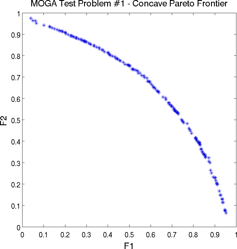
Fig. 50 Multiple objective genetic algorithm (MOGA) example: Pareto front showing trade-offs between functions f1 and f2.
Optimization with User-specified or Automatic Scaling
Some optimization problems involving design variables, objective functions, or constraints on vastly different scales may be solved more efficiently if these quantities are adjusted to a common scale (typically on the order of unity). With any optimizer (or least squares solver described in Nonlinear Least Squares), user-specified characteristic value scaling may be applied to any of continuous design variables, functions/residuals, nonlinear inequality and equality constraints, and linear inequality and equality constraints. Automatic scaling is available for variables or responses with one- or two-sided bounds or equalities and may be combined with user-specified scaling values. Logarithmic (\(\log_{10}\)) scaling is available and may also be combined with characteristic values. Log scaling is not available for linear constraints. Moreover, when continuous design variables are log scaled, linear constraints are not permitted in the problem formulation. Discrete variable scaling is not supported.
Scaling is enabled on a per-method basis for optimizers and calibration
(least squares and Bayesian) methods by including the scaling keyword in the
relevant method specification in the Dakota input file, e.g. for the
optpp_q_newton method. When scaling is
enabled, variables, functions, gradients, Hessians, etc., are
transformed such that the optimizer iterates in the scaled
variable/response space. Evaluations of the computational model
as specified in the interface are performed in the original problem
scale, alleviating the need to rewrite the interface
to the simulation code to perform scaling. When the scaling keyword is
absent form the method block, all scale type and value specifications
in the variables and responses blocks are ignored. Dakota prints
scaling initialization and diagnostic information to the console when
the output verbosity is set above normal.
Scaling for a particular variable or response type is enabled through
their scales, scale_types and related specifications (drill down
into variables or responses). Valid options
for the string-valued specifications include ’value’, ’auto’, or
’log’, for characteristic value, automatic, or logarithmic scaling,
respectively (although not all types are valid for scaling all
entities). If a single string is specified with any of these keywords it
will apply to each component of the relevant vector, e.g., with
continuous_design = 3,
scale_types = 'value' will
enable characteristic value scaling for each of the 3 continuous design
variables.
One may specify no, one, or a vector of characteristic scale values
through the scales specifications. These characteristic values are required for
’value’, and optional for ’auto’ and ’log’. If scales are
specified, but not scale types, value scaling is assumed. As with types,
if a single value is specified with any of these keywords it will apply
to each component of the relevant vector, e.g., if scales=3.4 is specified for
continuous design variables, Dakota will apply a characteristic scaling
value of 3.4 to each continuous design variable.
When scaling is enabled, the following procedures determine the
transformations used to scale each component of a variables or response
vector. A warning is issued if scaling would result in division by a
value smaller in magnitude than 1.0e10*DBL_MIN. User-provided values
violating this lower bound are accepted unaltered, whereas for
automatically calculated scaling, the lower bound is enforced.
No
scalesand noscale_types`specified for this component (variable or response type): no scaling performed on this component.Characteristic value (
’value’): the corresponding quantity is scaled (divided) by the required characteristic value provided in the corresponding specification, and bounds are adjusted as necessary. If the value is negative, the sense of inequalities are changed accordingly.Automatic (
’auto’): First, any characteristic values from the optional corresponding specification are applied. Then, automatic scaling will be attempted according to the following scheme:two-sided bounds scaled into the interval \([0,1]\);
one-sided bounds or targets are scaled by a characteristic value to move the bound or target to 1, and the sense of inequalities are changed if necessary;
no bounds or targets: no automatic scaling possible for this component
Automatic scaling is not available for objective functions nor least squares terms since they lack bound constraints. Further, when automatically scaled, linear constraints are scaled by characteristic values only, not affinely scaled into \([0,1]\).
Logarithmic (
’log’): First, any characteristic values from the optionalscalesspecification are applied. Then, \(\log_{10}\) scaling is applied. Logarithmic scaling is not available for linear constraints. Further, when continuous design variables are log scaled, linear constraints are not allowed.
Scaling for linear constraints specified through linear_inequality_scales
or linear_equality_scales is applied after
any (user-specified or automatic) continuous variable scaling. For
example, for scaling mapping unscaled continuous design variables
\(x\) to scaled variables \(\tilde{x}\):
where \(x^j_M\) is the final component multiplier and \(x^j_O\) the offset, we have the following matrix system for linear inequality constraints
and user-specified or automatically computed scaling multipliers are applied to this final transformed system, which accounts for any continuous design variable scaling. When automatic scaling is in use for linear constraints they are linearly scaled by characteristic values only, not affinely scaled into the interval \([0,1]\).
Scaling Example
Listing 53
demonstrates the use of several scaling keywords for the Rosenbrock
optimization problem. The first continuous design variable x1 is scaled by
a characteristic value of 4.0, and the second, x2, is scaled by 0.1 then logarithmically.
The objective function will be scaled by a factor of 50.0. Note that not only do the
scales and scale_types keywords appear in the variables and responses blocks;
the scaling keyword is also present in the method block. Both are necessary for scaling
to occur.
dakota/share/dakota/examples/users/rosen_opt_scaled.in# Dakota Input File: rosen_opt_scaled.in
environment
tabular_data
tabular_data_file = 'rosen_opt_scaled.dat'
method
conmin_frcg
scaling
output verbose
model
single
variables
continuous_design = 2
initial_point -1.2 1.0
lower_bounds -2.0 0.001
upper_bounds 2.0 2.0
descriptors 'x1' "x2"
scale_types = 'value' 'log'
scales = 4.0 0.1
interface
analysis_drivers = 'rosenbrock'
direct
responses
objective_functions = 1
primary_scale_types = 'value'
primary_scales = 50.0
analytic_gradients
no_hessians
Optimization Usage Guidelines
In selecting an optimization method, important considerations include the type of variables in the problem (continuous, discrete, mixed), whether a global search is needed or a local search is sufficient, and the required constraint support (unconstrained, bound constrained, or generally constrained). Less obvious, but equally important, considerations include the efficiency of convergence to an optimum (i.e., convergence rate) and the robustness of the method in the presence of challenging design space features (e.g., nonsmoothness, simulation failures).
Table 12 provides a convenient reference for choosing an optimization method or strategy to match the characteristics of the user’s problem. With respect to constraint support, it should be understood that the methods with more advanced constraint support are also applicable to the lower constraint support levels; they are listed only at their highest level of constraint support for brevity.
Method Classification |
Desired Problem Characteristics |
Applicable Methods |
|---|---|---|
Gradient-Based Local |
No constraints |
|
bound constraints |
||
bound constraints, linear and nonlinear constraints |
|
|
bound constraints, linear and nonlinear constraints; multiobjective |
||
Gradient-Based Global |
bound constraints, linear and nonlinear constraints |
|
Derivative-Free Local |
bound constraints |
|
bound constraints, nonlinear constraints |
||
bound constraints, linear and nonlinear constraints |
||
discrete variables; bound constraints, nonlinear constraints |
||
Derivative-Free Global |
bound constraints |
|
bound constraints, nonlinear constraints |
||
bound constraints, linear and nonlinear constraints |
||
discrete variables; bound constraints, nonlinear constraints |
||
discrete variables; bound constraints, linear and nonlinear constraints |
||
discrete variables; bound constraints, linear and nonlinear constraints; multiobjective |
Note
Gradient-based methods require continuous variables and differentiable (smooth) responses. Non-smooth objective functions can be optimized using derivative-free methods. All of Dakota’s optimization methods permit continous design variables; those that are compatible with discrete variables are so indicated in the table.
Gradient-based Methods
Gradient-based optimization methods are highly efficient, with the best convergence rates of all of the optimization methods. If analytic gradient and Hessian information can be provided by an application code, a full Newton method will provide quadratic convergence rates near the solution. More commonly, only gradient information is available and a quasi-Newton method is chosen in which the Hessian information is approximated from an accumulation of gradient data. In this case, superlinear convergence rates can be obtained. First-order methods, such as the Method of Feasible Directions, may achieve only a linear rate of convergence, which may entail more iterations, but potentially at a lower cost per iteration associated with Hessian calculations. These characteristics make gradient-based optimization the methods of choice when the problem is smooth, unimodal, and well-behaved. However, when the problem exhibits nonsmooth, discontinuous, or multimodal behavior, these methods can also be the least robust since inaccurate gradients will lead to bad search directions, failed line searches, and early termination, and the presence of multiple minima will be missed.
Thus, for gradient-based optimization, a critical factor is the gradient accuracy. Analytic gradients are ideal, but are often unavailable. For many engineering applications, a finite difference method will be used by the optimization algorithm to estimate gradient values. Dakota allows the user to select the step size for these calculations, as well as choose between forward-difference and central-difference algorithms. The finite difference step size should be selected as small as possible, to allow for local accuracy and convergence, but not so small that the steps are “in the noise.” This requires an assessment of the local smoothness of the response functions using, for example, a parameter study method. Central differencing, in general, will produce more reliable gradients than forward differencing, but at roughly twice the expense.
ROL has traditionally been developed and applied to problems with analytic gradients (and Hessians). Nonetheless, ROL can be used with Dakota-provided finite-differencing approximations to the gradient of both objective and constraints. However, a user relying on such approximations is advised to resort to alternative optimizers such as DOT until performance of ROL improves in future releases.
We offer the following recommendations in deciding upon a suitable gradient-based method for a given problem
For unconstrained and bound-constrained problems, conjugate gradient-based methods exhibit the best scalability for large-scale problems (1,000+ variables). These include the Polak-Ribiere conjugate gradient method (
optpp_cg), ROL’s trust-region method with truncated conjugate gradient subproblem solver (rol), and the Fletcher-Reeves conjugate gradient method (conmin_frcganddot_frcg). These methods also provide good performance for small- to intermediate-sized problems. Note that due to performance issues, users relying on finite-differencing approximations to the gradient of the objective function are advised to resort to alternative optimizers such as DOT until performance of ROL improves in future releases.For constrained problems, with large number of constraints with respect to number of variables, Method of Feasible Directions methods (
conmin_mfdanddot_mmfd) and Sequential Quadratic Programming methods (nlpql_sqpandnpsol_sqp) exhibit good performance (relatively fast convergence rates). The quasi-Newton methodoptpp_q_newtonshow moderate performance for constrained problems across all scales.
Note
We have observed weak convergence rates while using npsol_sqp for certain
problems with equality constraints.
Non-gradient-based Methods
Nongradient-based methods exhibit much slower convergence rates for finding an optimum, and as a result, tend to be much more computationally demanding than gradient-based methods. Nongradient local optimization methods, such as pattern search algorithms, often require from several hundred to a thousand or more function evaluations, depending on the number of variables, and nongradient global optimization methods such as genetic algorithms may require from thousands to tens-of-thousands of function evaluations. Clearly, for nongradient optimization studies, the computational cost of the function evaluation must be relatively small in order to obtain an optimal solution in a reasonable amount of time. In addition, nonlinear constraint support in nongradient methods is an open area of research and, while supported by many nongradient methods in Dakota, is not as refined as constraint support in gradient-based methods. However, nongradient methods can be more robust and more inherently parallel than gradient-based approaches. They can be applied in situations were gradient calculations are too expensive or unreliable. In addition, some nongradient-based methods can be used for global optimization which gradient-based techniques, by themselves, cannot. For these reasons, nongradient-based methods deserve consideration when the problem may be nonsmooth, multimodal, or poorly behaved.
Surrogate-based Methods
The effectiveness or efficiency of optimization (and calibration)
methods can often be improved through the use of surrogate models. Any
Dakota optimization method can be used with a (build-once) global
surrogate by specifying the id_model of a global surrogate
model with the optimizer’s model_pointer keyword. This approach can
be used with surrogates trained from (static) imported data or trained
online using a Dakota Design of Experiments submethod.
When online query of the underlying truth model at new design values is possible, tailored/adaptive surrogate-based methods may perform better as they refine the surrogate as the optimization progresses. The surrogate-based local approach (see Surrogate-based Local Minimization) brings the efficiency of gradient-based optimization/least squares methods to nonsmooth or poorly behaved problems by smoothing noisy or discontinuous response results with a data fit surrogate model (e.g., a quadratic polynomial) and then minimizing on the smooth surrogate using efficient gradient-based techniques. The surrogate-based global approach (see Surrogate-based Global Minimization) similarly employs optimizers/least squares methods with surrogate models, but rather than localizing through the use of trust regions, seeks global solutions using global methods. And the efficient global approach uses the specific combination of Gaussian process surrogate models and the DIRECT global optimizer. Similar to these surrogate-based approaches, the hybrid and multistart optimization component-based algorithms seek to bring the efficiency of gradient-based optimization methods to global optimization problems. In the former case, a global optimization method can be used for a few cycles to locate promising regions and then local gradient-based optimization is used to efficiently converge on one or more optima. In the latter case, a stratification technique is used to disperse a series of local gradient-based optimization runs through parameter space. Without surrogate data smoothing, however, these strategies are best for smooth multimodal problems. The Hybrid Minimization and Multistart Local Minimization sections provide more information on these approaches.
Specifying Mixed Bounds: When solving constrained optimization
problems, optimization (and calibration) solvers will use
*lower_bounds and *upper_bounds information from individual
variable types, linear constraints (see variables), and
nonlinear constraints (see responses). For most optimization
solvers, a nonexistent upper bound can be specified by using a value
greater than the “big bound size” constant (1.e+30 for continuous
variables, 1.e+9 for discrete integer variables) and a nonexistent
lower bound can be specified by using a value less than the negation
of these constants (-1.e+30 for continuous, -1.e+9 for discrete
integer). Not all optimizers currently support this feature, e.g., DOT
and CONMIN will treat these large bound values as actual variable
bounds, but this should not be problematic in practice.
Optimization Third Party Libraries
As mentioned previously, Dakota serves as a delivery vehicle for a number third-party optimization libraries. The packages are listed here along with the license status and web page where available.
CONMIN (
conmin_methods) License: Public Domain (NASA).DOT (
dot_methods) License: commercial; website: Vanderplaats Research and Development, http://www.vrand.com.
Note
The DOT library is Not included in the open source version of Dakota. Sandia National Laboratories and Los Alamos National Laboratory have limited seats for DOT. Other users may obtain their own copy of DOT and compile it with the Dakota source code.
HOPSPACK (
asynch_pattern_search) License: LGPL; web page: https://software.sandia.gov/trac/hopspack.JEGA (
soga,moga) License: LGPLNCSUOpt (
ncsu_direct) License: MITNLPQL (
nlpql_methods) License: commercial; website: Prof. Klaus Schittkowski, http://www.uni-bayreuth.de/departments/math/~kschittkowski/nlpqlp20.htm).
Note
The NLPQL library is not included in the open source version of Dakota. Users may obtain their own copy of NLPQLP and compile it with the Dakota source code.
NPSOL (
npsol_methods) License: commercial; website: Stanford Business Software http://www.sbsi-sol-optimize.com.
Note
The NPSOL library is not included in the open source version of Dakota. Sandia National Laboratories, Lawrence Livermore National Laboratory, and Los Alamos National Laboratory all have site licenses for NPSOL. Other users may obtain their own copy of NPSOL and compile it with the Dakota source code.*
NOMAD (
mesh_adaptive_search) License: LGPL; website: http://www.gerad.ca/NOMAD/Project/Home.html.OPT++ (
optpp_methods) License: LGPL; website: http://csmr.ca.sandia.gov/opt++.ROL (
rol) License: BSD; website: https://trilinos.org/packages/rol.SCOLIB (
coliny_methods) License: BSD; website: https://software.sandia.gov/trac/acro/wiki/Packages.
Video Resources
Title |
Link |
Resources |
|---|---|---|
Optimization |
|