Parameter Studies
Overview
Dakota parameter studies explore the effect of parametric changes on simulation models by computing response data sets at a selection of points in the parameter space, yielding one type of sensitivity analysis. (Contrast these with DACE-based sensitivity analysis.) The selection of points is deterministic, whether structured or user-specified, in each of the four available parameter study methods:
Vector: Performs a parameter study along a line between any two points in an \(n\)-dimensional parameter space, where the user specifies the number of steps used in the study.
List: The user supplies a list of points in an \(n\)-dimensional space where Dakota will evaluate response data from the simulation code.
Centered: Given a point in an \(n\)-dimensional parameter space, this method evaluates nearby points along the coordinate axes of the parameter space. The user selects the number of steps and the step size.
Multidimensional: Forms a regular lattice or hypergrid in an \(n\)-dimensional parameter space, where the user specifies the number of intervals used for each parameter.
When used in parameter studies, the response data sets are not linked to any specific interpretation, so they may consist of any allowable specification from the responses keyword block, i.e., objective and constraint functions, least squares terms and constraints, or generic response functions. This allows the use of parameter studies in alternation with optimization, least squares, and uncertainty quantification studies with only minor modification to the input file. In addition, the response data sets may include gradients and Hessians of the response functions, which will be catalogued by the parameter study. This allows for several different approaches to “sensitivity analysis”: (1) the variation of function values over parameter ranges provides a global assessment as to the sensitivity of the functions to the parameters, (2) derivative information can be computed numerically, provided analytically by the simulator, or both (mixed gradients) in directly determining local sensitivity information at a point in parameter space, and (3) the global and local assessments can be combined to investigate the variation of derivative quantities through the parameter space by computing sensitivity information at multiple points.
Parameter studies can also be used for investigating nonsmoothness in simulation response variations (so that models can be refined or finite difference step sizes can be selected for computing numerical gradients), interrogating problem areas in the parameter space, or performing simulation code verification (verifying simulation robustness) through parameter ranges of interest. A parameter study can also be used in coordination with minimization methods as either a pre-processor (to identify a good starting point) or a post-processor (for post-optimality analysis).
Parameter study methods will iterate any combination of design,
uncertain, and state variables (possibly filtered by the
active keyword) defined over continuous and discrete
domains into any set of responses (any function, gradient, and Hessian
definition). Parameter studies draw no distinction among the different
types of continuous variables (design, uncertain, or state) or among
the different types of response functions. They simply pass all of the
variables defined in the variables specification into the interface,
from which they expect to retrieve all of the responses defined in the
responses specification. As described in Active Variables for Derivatives, when
gradient and/or Hessian information is being catalogued in the
parameter study, it is assumed that derivative components will be
computed with respect to all of the continuous variables (continuous
design, continuous uncertain, and continuous state variables)
specified, since derivatives with respect to discrete variables are
assumed to be undefined. The specification of initial values or bounds
is important for parameter studies.
Initial Values
The vector and centered parameter studies use the initial values of
the variables from the variables keyword block as the
starting point and the central point of the parameter studies,
respectively. These parameter study starting values for design,
uncertain, and state variables are referenced in the following
sections using the identifier “Initial Values.”
In the case of design variables, the initial_point is used, and in
the case of state variables, the initial_state is used. In the
case of uncertain variables, initial values not specified by an
initial_point are inferred from the distribution specification:
all uncertain initial values are set to their means, correcting as
needed. For example, mean values for bounded normal and bounded
lognormal are repaired as needed to satisfy the specified distribution
bounds, mean values for discrete integer range distributions are
rounded down to the nearest integer, and mean values for discrete set
distributions are rounded to the nearest set value. See the
initial_* children of each type of variables for
additional details on default values.
Bounds
The multidimensional parameter study uses the bounds of the variables
from the variables keyword block to define the range of
parameter values to study. In the case of design and state variables,
the lower_bounds and upper_bounds specifications are used (see
the keyword documentation for default values when lower_bounds or
upper_bounds are unspecified). In the case of uncertain variables,
these values are either drawn or inferred from the distribution
specification. Distribution lower and upper bounds can be drawn
directly from required bounds specifications for uniform, loguniform,
triangular, and beta distributions, as well as from optional bounds
specifications for normal and lognormal. Distribution bounds are
implicitly defined for histogram bin, histogram point, and interval
variables (from the extreme values within the bin/point/interval
specifications) as well as for binomial (0 to
num_trials) and
hypergeometric (0 to
min(num_drawn,
selected_population))
variables. Finally, distribution bounds are inferred for normal and
lognormal if optional bounds are unspecified, as well as for
exponential, gamma, gumbel, frechet, weibull, poisson, negative
binomial, and geometric (which have no bounds specifications); these
bounds are \([0, \mu + 3 \sigma]\) for exponential, gamma,
frechet, weibull, poisson, negative binomial, geometric, and
unspecified lognormal, and \([\mu - 3\sigma, \mu + 3\sigma]\) for
gumbel and unspecified normal.
Vector Parameter Study
The vector parameter study computes response data sets at selected intervals along an \(n\)-dimensional vector in parameter space. This capability encompasses both single-coordinate parameter studies (to study the effect of a single variable on a response set) as well as multiple coordinate vector studies (to investigate the response variations along some arbitrary vector; e.g., to investigate a search direction failure).
Vector studies use either
final_point(vector of reals) withnum_steps(integer), orstep_vector(vector of reals) withnum_steps(integer)
in conjunction with the Initial Values to define the vector and steps of the parameter study.
In both of these cases, the Initial Values are used as the parameter study starting point and the specification selection above defines the orientation of the vector and the increments to be evaluated along the vector. In the former case, the vector from initial to final point is partitioned by the number of steps, and in the latter case, the step vector is added number of steps times. Thus the number of evaluations is \(\mathtt{num\_steps} +1\).
Note
For discrete range variables, both
final_point and
step_vector are specified in
the actual numerical values. For integer- or real-valued discrete
sets, final_point is
specified in the actual numerical values, while for discrete string
variable it is given using a zero-based index into the sorted
admissible string values. For all discrete set variables,
step_vector must specify
index offsets for the (ordered, unique) set.
Example 1: Three continuous parameters with initial values of
(1.0, 1.0, 1.0), num_steps = 4,
and either final_point = (1.0,
2.0, 1.0) or step_vector = (0,
.25, 0):
Parameters for function evaluation 1:
                      1.0000000000e+00 c1
                      1.0000000000e+00 c2
                      1.0000000000e+00 c3
Parameters for function evaluation 2:
                      1.0000000000e+00 c1
                      1.2500000000e+00 c2
                      1.0000000000e+00 c3
Parameters for function evaluation 3:
                      1.0000000000e+00 c1
                      1.5000000000e+00 c2
                      1.0000000000e+00 c3
Parameters for function evaluation 4:
                      1.0000000000e+00 c1
                      1.7500000000e+00 c2
                      1.0000000000e+00 c3
Parameters for function evaluation 5:
                      1.0000000000e+00 c1
                      2.0000000000e+00 c2
                      1.0000000000e+00 c3
Example 2: Two continuous parameters with initial values of (1.0,
1.0), one discrete range parameter with initial value of 5, one
discrete real set parameter with set values of (10., 12., 18., 30.,
50.) and initial value of 10.,
num_steps = 4, and either
final_point = (2.0, 1.4, 13,
50.) or step_vector = (.25, .1,
2, 1):
Parameters for function evaluation 1:
                      1.0000000000e+00 c1
                      1.0000000000e+00 c2
                                     5 di1
                      1.0000000000e+01 dr1
Parameters for function evaluation 2:
                      1.2500000000e+00 c1
                      1.1000000000e+00 c2
                                     7 di1
                      1.2000000000e+01 dr1
Parameters for function evaluation 3:
                      1.5000000000e+00 c1
                      1.2000000000e+00 c2
                                     9 di1
                      1.8000000000e+01 dr1
Parameters for function evaluation 4:
                      1.7500000000e+00 c1
                      1.3000000000e+00 c2
                                    11 di1
                      3.0000000000e+01 dr1
Parameters for function evaluation 5:
                      2.0000000000e+00 c1
                      1.4000000000e+00 c2
                                    13 di1
                      5.0000000000e+01 dr1
See Example: Vector Parameter Study with Rosenbrock for a more detailed vector parameter study example.
List Parameter Study
The list parameter study computes response data sets at selected points in parameter space. These points are explicitly specified by the user and are not confined to lie on any line or surface. Thus, this parameter study provides a general facility that supports the case where the desired set of points to evaluate does not fit the prescribed structure of the vector, centered, or multidimensional parameter studies.
The principal user input is via
list_of_points which lists the
requested parameter sets in succession. The list parameter study
simply performs a simulation for the first parameter set (the first
\(n\) entries in the list), followed by a simulation for the next
parameter set (the next \(n\) entries), and so on, until the list
of points has been exhausted. Since the Initial Values will not be
used, they need not be specified.
Note
The list values for discrete string set variables must be specified by zero-based indices into the ordered list of admissible strings.
In contrast, for integer- or real-valued discrete range or discrete set variables, list values are specified using the actual numerical values (not set indices).
A specification that would result in the same parameter sets as in the second vector parameter study example is:
list_of_points = 1.0  1.0  5 10.
                 1.25 1.1  7 12.
                 1.5  1.2  9 18.
                 1.75 1.3 11 30.
                 2.0  1.4 13 50.
For convenience, the points to be evaluated may instead be imported
from a file using
import_points_file, e.g.,
import_points_file 'listpstudy.dat', where the file
listpstudy.dat may be in freeform or annotated format. The points for each evaluation must be given
in input specification order, with both active and inactive variables
by default.
Centered Parameter Study
The centered parameter study study executes multiple coordinate-based parameter studies, one per parameter, centered at the specified Initial Values. This can help investigate function contours in the vicinity of a specific point. For example, after computing an optimum design, this capability could be used for post-optimality analysis in verifying that the computed solution is actually at a minimum or constraint boundary and in investigating the shape of this minimum or constraint boundary.
This method requires
step_vector (list of reals)
and steps_per_variable (list
of integers) specifications, where the former specifies the size of
the increments per variable and the latter specifies the number of
increments per variable for each of the positive and negative step
directions. (These steps are applied sequentially, not all at once as
in the vector study.)
Note
Similar to the the vector study
step_vector includes
actual variable steps for continuous and discrete range variables,
but employs index offsets for discrete set variables (integer,
string, or real).
For example, with Initial Values of (1.0, 1.0), a
step_vector of (0.1, 0.1),
and a steps_per_variable of
(2, 2), the center point is evaluated followed by four function
evaluations (two negative deltas and two positive deltas) per
variable:
Parameters for function evaluation 1:
                      1.0000000000e+00 d1
                      1.0000000000e+00 d2
Parameters for function evaluation 2:
                      8.0000000000e-01 d1
                      1.0000000000e+00 d2
Parameters for function evaluation 3:
                      9.0000000000e-01 d1
                      1.0000000000e+00 d2
Parameters for function evaluation 4:
                      1.1000000000e+00 d1
                      1.0000000000e+00 d2
Parameters for function evaluation 5:
                      1.2000000000e+00 d1
                      1.0000000000e+00 d2
Parameters for function evaluation 6:
                      1.0000000000e+00 d1
                      8.0000000000e-01 d2
Parameters for function evaluation 7:
                      1.0000000000e+00 d1
                      9.0000000000e-01 d2
Parameters for function evaluation 8:
                      1.0000000000e+00 d1
                      1.1000000000e+00 d2
Parameters for function evaluation 9:
                      1.0000000000e+00 d1
                      1.2000000000e+00 d2
This set of points in parameter space is depicted in Fig. 35
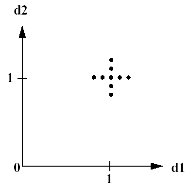
Fig. 35 Example centered parameter study.
Multidimensional Parameter Study
The multidimensional parameter study computes response data sets for an \(n\)-dimensional hypergrid of points. Each variable is partitioned into equally spaced intervals between its upper and lower bounds, and each combination of the values defined by these partitions is evaluated. The number of function evaluations performed in the study is:
where the partitions keyword
gives an integer list of the number of partitions for each variable
(i.e., \(\mathtt{partitions}_{i}\)). Since the Initial Values will
not be used, they need not be specified.
Note
As for the vector and centered studies, partitioning occurs using the actual variable values for continuous and discrete range variables, but occurs within the space of valid indices for discrete set variables (integer, string, or real).
In a two variable example problem with \(d1 \in [0, 2]\) and
\(d2 \in [0,3]\) (as defined by the upper and lower bounds from
the variables specification) and with
partitions = (2, 3), the
interval [0, 2] is divided into two equal-sized partitions and the
interval [0, 3] is divided into three equal-sized partitions. This
two-dimensional grid, shown in Fig. 36, would result
in the following twelve function evaluations:
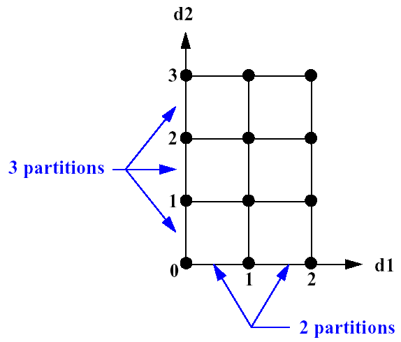
Fig. 36 Example multidimensional parameter study
Parameters for function evaluation 1:
                      0.0000000000e+00 d1
                      0.0000000000e+00 d2
Parameters for function evaluation 2:
                      1.0000000000e+00 d1
                      0.0000000000e+00 d2
Parameters for function evaluation 3:
                      2.0000000000e+00 d1
                      0.0000000000e+00 d2
Parameters for function evaluation 4:
                      0.0000000000e+00 d1
                      1.0000000000e+00 d2
Parameters for function evaluation 5:
                      1.0000000000e+00 d1
                      1.0000000000e+00 d2
Parameters for function evaluation 6:
                      2.0000000000e+00 d1
                      1.0000000000e+00 d2
Parameters for function evaluation 7:
                      0.0000000000e+00 d1
                      2.0000000000e+00 d2
Parameters for function evaluation 8:
                      1.0000000000e+00 d1
                      2.0000000000e+00 d2
Parameters for function evaluation 9:
                      2.0000000000e+00 d1
                      2.0000000000e+00 d2
Parameters for function evaluation 10:
                      0.0000000000e+00 d1
                      3.0000000000e+00 d2
Parameters for function evaluation 11:
                      1.0000000000e+00 d1
                      3.0000000000e+00 d2
Parameters for function evaluation 12:
                      2.0000000000e+00 d1
                      3.0000000000e+00 d2
See Two-Dimensional Grid Parameter Study for a more detailed example of a multi-dimensional parameter study.
Parameter Study Usage Guidelines
Parameter studies, classical design of experiments (DOE), design/analysis of computer experiments (DACE), and sampling methods share the purpose of exploring the parameter space. Parameter Studies are recommended for simple studies with defined, repetitive structure. A local sensitivity analysis or an assessment of the smoothness of a response function is best addressed with a vector or centered parameter study. A multi-dimensional parameter study may be used to generate grid points for plotting response surfaces. For guidance on DACE and sampling methods, in contrast to parameter studies, see DOE Usage Guidelines and especially Table 6, which clarifies the different purposes of the method types.
Example: Vector Parameter Study with Rosenbrock
This section demonstrates a vector parameter study on the Rosenbrock test function described in Rosenbrock Test Problem. A similar example of a multidimensional parameter study is shown in Two-Dimensional Grid Parameter Study.
A vector parameter study is a study between any two design points in
an \(n\)-dimensional parameter space. An input file for the
vector parameter study is shown in
Listing 27. The primary differences
between this input file and the input file for the multidimensional
parameter study are found in the variables and method sections. In
the variables section, the keywords for the bounds are removed and
replaced with the keyword initial_point that specifies the
starting point for the parameter study. In the method section, the
vector_parameter_study keyword is used. The
final_point keyword indicates
the stopping point for the parameter study, and
num_steps specifies the number
of steps taken between the initial and final points in the parameter
study.
dakota/share/dakota/examples/users/rosen_ps_vector.in# Dakota Input File: rosen_ps_vector.in
environment
tabular_data
tabular_data_file = 'rosen_ps_vector.dat'
method
vector_parameter_study
final_point = 1.1 1.3
num_steps = 10
model
single
variables
continuous_design = 2
initial_point -0.3 0.2
descriptors 'x1' "x2"
interface
analysis_drivers = 'rosenbrock'
direct
responses
objective_functions = 1
no_gradients
no_hessians
Fig. 37 shows the legacy X Windows-based graphics output created by Dakota, which can be useful for visualizing the results. Fig. 38 shows the locations of the 11 sample points generated in this study. The parameter study starts within the banana-shaped valley, marches up the side of the hill, and then returns to the valley.
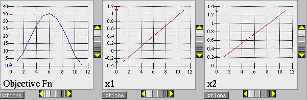
Fig. 37 Iteration history for Rosenbrock vector parameter study
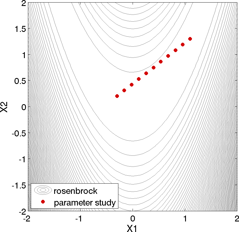
Fig. 38 Evaluation points (red dots) for Rosenbrock vector parameter study