Surrogate-Based Local Minimization
A generally-constrained nonlinear programming problem takes the form
where \({\bf x} \in \Re^n\) is the vector of design variables, and \(f\), \({\bf g}\), and \({\bf h}\) are the objective function, nonlinear inequality constraints, and nonlinear equality constraints, respectively. (Any linear constraints are not approximated and may be added without modification to all formulations). Individual nonlinear inequality and equality constraints are enumerated using \(i\) and \(j\), respectively (e.g., \(g_i\) and \(h_j\)). The corresponding surrogate-based optimization (SBO) algorithm may be formulated in several ways and applied to either optimization or least-squares calibration problems. In all cases, SBO solves a sequence of \(k\) approximate optimization subproblems subject to a trust region constraint \(\Delta^k\); however, many different forms of the surrogate objectives and constraints in the approximate subproblem can be explored. In particular, the subproblem objective may be a surrogate of the original objective or a surrogate of a merit function (most commonly, the Lagrangian or augmented Lagrangian), and the subproblem constraints may be surrogates of the original constraints, linearized approximations of the surrogate constraints, or may be omitted entirely. Each of these combinations is shown in Table 17, where some combinations are marked inappropriate, others acceptable, and the remaining are common.
Original Objective |
Lagrangian |
Augmented Lagrangian |
|
|---|---|---|---|
No constraints |
inappropriate |
acceptable |
TRAL |
Linearized constraints |
acceptable |
SQP-like |
acceptable |
Original constraints |
Direct surrogate |
acceptable |
IPTRSAO |
Initial approaches to nonlinearly-constrained SBO optimized an approximate merit function which incorporated the nonlinear constraints [ALG+00, RRW98]:
where the surrogate merit function is denoted as \(\hat \Phi({\bf x})\), \({\bf x}_c\) is the center point of the trust region, and the trust region is truncated at the global variable bounds as needed. The merit function to approximate was typically chosen to be a standard implementation [GMW81, NJ99, Van84] of the augmented Lagrangian merit function (see Eqs. (243) and (244)), where the surrogate augmented Lagrangian is constructed from individual surrogate models of the objective and constraints (approximate and assemble, rather than assemble and approximate). In Table 17, this corresponds to row 1, column 3, and is known as the trust-region augmented Lagrangian (TRAL) approach. While this approach was provably convergent, convergence rates to constrained minima have been observed to be slowed by the required updating of Lagrange multipliers and penalty parameters [PerezRW04]. Prior to converging these parameters, SBO iterates did not strictly respect constraint boundaries and were often infeasible. A subsequent approach (IPTRSAO [PerezRW04]) that sought to directly address this shortcoming added explicit surrogate constraints (row 3, column 3 in Table 17):
While this approach does address infeasible iterates, it still shares the feature that the surrogate merit function may reflect inaccurate relative weightings of the objective and constraints prior to convergence of the Lagrange multipliers and penalty parameters. That is, one may benefit from more feasible intermediate iterates, but the process may still be slow to converge to optimality. The concept of this approach is similar to that of SQP-like SBO approaches [ALG+00] which use linearized constraints:
in that the primary concern is minimizing a composite merit function of the objective and constraints, but under the restriction that the original problem constraints may not be wildly violated prior to convergence of Lagrange multiplier estimates. Here, the merit function selection of the Lagrangian function (row 2, column 2 in Table 17; see also Eq. (242)) is most closely related to SQP, which includes the use of first-order Lagrange multiplier updates (Eq. (248)) that should converge more rapidly near a constrained minimizer than the zeroth-order updates (Eqs. (245) and (246)) used for the augmented Lagrangian.
All of these previous constrained SBO approaches involve a recasting of the approximate subproblem objective and constraints as a function of the original objective and constraint surrogates. A more direct approach is to use a formulation of:
This approach has been termed the direct surrogate approach since it optimizes surrogates of the original objective and constraints (row 3, column 1 in Table 17) without any recasting. It is attractive both from its simplicity and potential for improved performance, and is the default approach taken in Dakota. Other Dakota defaults include the use of a filter method for iterate acceptance, an augmented Lagrangian merit merit function), Lagrangian hard convergence assessment), and no constraint relaxation.
While the formulation of Eq. (235) (and others from row 1 in Table 17) can suffer from infeasible intermediate iterates and slow convergence to constrained minima, each of the approximate subproblem formulations with explicit constraints (Eqs. (236)-(238), and others from rows 2-3 in Table 17) can suffer from the lack of a feasible solution within the current trust region. Techniques for dealing with this latter challenge involve some form of constraint relaxation. Homotopy approaches [PerezEaR04, PerezRW04] or composite step approaches such as Byrd-Omojokun [Omo89], Celis-Dennis-Tapia [CDT85], or MAESTRO [ALG+00] may be used for this purpose (see Constraint relaxation).
After each of the \(k\) iterations in the SBO method, the predicted step is validated by computing \(f({\bf x}^k_\ast)\), \({\bf g}({\bf x}^k_\ast)\), and \({\bf h}({\bf x}^k_\ast)\). One approach forms the trust region ratio \(\rho^k\) which measures the ratio of the actual improvement to the improvement predicted by optimization on the surrogate model. When optimizing on an approximate merit function (Eqs. (235)-(237)), the following ratio is natural to compute
The formulation in Eq. (238) may also form a merit function for computing the trust region ratio; however, the omission of this merit function from explicit use in the approximate optimization cycles can lead to synchronization problems with the optimizer.
Once computed, the value for \(\rho^k\) can be used to define the step acceptance and the next trust region size \(\Delta^{k+1}\) using logic similar to that shown in Table 18. Typical factors for shrinking and expanding are 0.5 and 2.0, respectively, but these as well as the threshold ratio values are tunable parameters in the algorithm (see surrogate-sased method controls in the keyword reference area In addition, the use of discrete thresholds is not required, and continuous relationships using adaptive logic can also be explored [WR98a, WR98b]. Iterate acceptance or rejection completes an SBO cycle, and the cycles are continued until either soft or hard convergence criteria are satisfied.
Ratio Value |
Surrogate Accuracy |
Iterate Acceptance |
Trust Region Sizing |
|---|---|---|---|
\(\rho^k \le 0\) |
poor |
reject step |
shrink |
\(0 < \rho^k \le 0.25\) |
marginal |
accept step |
shrink |
\(0.25 < \rho^k < 0.75\) or \(\rho^k > 1.25\) |
moderate |
accept step |
retain |
\(0.75 \le \rho^k \le 1.25\) |
good |
accept step |
expand |
Iterate acceptance logic
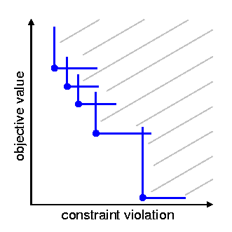
Fig. 82 Illustration of slanting filter
When a surrogate optimization is completed and the approximate solution has been validated, then the decision must be made to either accept or reject the step. The traditional approach is to base this decision on the value of the trust region ratio, as outlined previously in Table 18. An alternate approach is to utilize a filter method [FLT02], which does not require penalty parameters or Lagrange multiplier estimates. The basic idea in a filter method is to apply the concept of Pareto optimality to the objective function and constraint violations and only accept an iterate if it is not dominated by any previous iterate. Mathematically, a new iterate is not dominated if at least one of the following:
is true for all \(i\) in the filter, where \(c\) is a selected norm of the constraint violation. This basic description can be augmented with mild requirements to prevent point accumulation and assure convergence, known as a slanting filter [FLT02]. Fig. 82 illustrates the filter concept, where objective values are plotted against constraint violation for accepted iterates (blue circles) to define the dominated region (denoted by the gray lines). A filter method relaxes the common enforcement of monotonicity in constraint violation reduction and, by allowing more flexibility in acceptable step generation, often allows the algorithm to be more efficient.
The use of a filter method is compatible with any of the SBO formulations in Eqs. (235)-(238).
Merit functions
The merit function \(\Phi({\bf x})\) used in Eqs. (235)-(237), (239) may be selected to be a penalty function, an adaptive penalty function, a Lagrangian function, or an augmented Lagrangian function. In each of these cases, the more flexible inequality and equality constraint formulations with two-sided bounds and targets (Eqs. (234), (236)-(238)) have been converted to a standard form of \({\bf g}({\bf x}) \le 0\) and \({\bf h}({\bf x}) = 0\) (in Eqs. (240), (242)-(248)). The active set of inequality constraints is denoted as \({\bf g}^+\).
The penalty function employed in this paper uses a quadratic penalty with the penalty schedule linked to SBO iteration number
The adaptive penalty function is identical in form to Eq. (240), but adapts \(r_p\) using monotonic increases in the iteration offset value in order to accept any iterate that reduces the constraint violation.
The Lagrangian merit function is
for which the Lagrange multiplier estimation is discussed in Convergence Assessment. Away from the optimum, it is possible for the least squares estimates of the Lagrange multipliers for active constraints to be zero, which equates to omitting the contribution of an active constraint from the merit function. This is undesirable for tracking SBO progress, so usage of the Lagrangian merit function is normally restricted to approximate subproblems and hard convergence assessments.
The augmented Lagrangian employed in this paper follows the sign conventions described in [Van84]
where \(\psi\)(x) is derived from the elimination of slack variables for the inequality constraints. In this case, simple zeroth-order Lagrange multiplier updates may be used:
The updating of multipliers and penalties is carefully orchestrated [CGT00] to drive reduction in constraint violation of the iterates. The penalty updates can be more conservative than in Eq. (241), often using an infrequent application of a constant multiplier rather than a fixed exponential progression.
Convergence assessment
To terminate the SBO process, hard and soft convergence metrics are monitored. It is preferable for SBO studies to satisfy hard convergence metrics, but this is not always practical (e.g., when gradients are unavailable or unreliable). Therefore, simple soft convergence criteria are also employed which monitor for diminishing returns (relative improvement in the merit function less than a tolerance for some number of consecutive iterations).
To assess hard convergence, one calculates the norm of the projected gradient of a merit function whenever the feasibility tolerance is satisfied. The best merit function for this purpose is the Lagrangian merit function from Eq. (242). This requires a least squares estimation for the Lagrange multipliers that best minimize the projected gradient:
where gradient portions directed into active global variable bounds have been removed. This can be posed as a linear least squares problem for the multipliers:
where \({\bf A}\) is the matrix of active constraint gradients, \(\mbox{$\boldsymbol \lambda$}_g\) is constrained to be non-negative, and \(\mbox{$\boldsymbol \lambda$}_h\) is unrestricted in sign. To estimate the multipliers using non-negative and bound-constrained linear least squares, the NNLS and BVLS routines [LH74] from NETLIB are used, respectively.
Constraint relaxation
The goal of constraint relaxation is to achieve efficiency through the balance of feasibility and optimality when the trust region restrictions prevent the location of feasible solutions to constrained approximate subproblems (Eqs. (236)-(238), and other formulations from rows 2-3 in Table 17). The SBO algorithm starting from infeasible points will commonly generate iterates which seek to satisfy feasibility conditions without regard to objective reduction [PerezEaR04].
One approach for achieving this balance is to use relaxed constraints when iterates are infeasible with respect to the surrogate constraints. We follow Perez, Renaud, and Watson [PerezRW04], and use a global homotopy mapping the relaxed constraints and the surrogate constraints. For formulations in Eqs. (236) and (238) (and others from row 3 Table 17), the relaxed constraints are defined from
For Eq. (237) (and others from row 2 in Table 17), the original surrogate constraints \({\bf {\hat g}}^k({\bf x})\) and \({\bf {\hat h}}^k({\bf x})\) in Eqs. (249)-(250) are replaced with their linearized forms (\({\bf {\hat g}}^k({\bf x}^k_c) + \nabla {\bf {\hat g}}^k({\bf x}^k_c)^T ({\bf x} - {\bf x}^k_c)\) and \({\bf {\hat h}}^k({\bf x}^k_c) + \nabla {\bf {\hat h}}^k({\bf x}^k_c)^T ({\bf x} - {\bf x}^k_c)\), respectively). The approximate subproblem is then reposed using the relaxed constraints as
in place of the corresponding subproblems in Eqs. (236)-(238). Alternatively, since the relaxation terms are constants for the \(k^{th}\) iteration, it may be more convenient for the implementation to constrain \({\bf {\hat g}}^k({\bf x})\) and \({\bf {\hat h}}^k({\bf x})\) (or their linearized forms) subject to relaxed bounds and targets (\({\bf {\tilde g}}_l^k\), \({\bf {\tilde g}}_u^k\), \({\bf {\tilde h}}_t^k\)). The parameter \(\tau\) is the homotopy parameter controlling the extent of the relaxation: when \(\tau=0\), the constraints are fully relaxed, and when \(\tau=1\), the surrogate constraints are recovered. The vectors \({\bf b}_{g}, {\bf b}_{h}\) are chosen so that the starting point, \({\bf x}^0\), is feasible with respect to the fully relaxed constraints:
At the start of the SBO algorithm, \(\tau^0=0\) if \({\bf x}^0\) is infeasible with respect to the unrelaxed surrogate constraints; otherwise \(\tau^0=1\) (i.e., no constraint relaxation is used). At the start of the \(k^{th}\) SBO iteration where \(\tau^{k-1} < 1\), \(\tau^k\) is determined by solving the subproblem
starting at \(({\bf x}^{k-1}_*, \tau^{k-1})\), and then adjusted as follows:
The adjustment parameter \(0 < \alpha < 1\) is chosen so that that the feasible region with respect to the relaxed constraints has positive volume within the trust region. Determining the optimal value for \(\alpha\) remains an open question and will be explored in future work.
After \(\tau^k\) is determined using this procedure, the problem in Eq. (251) is solved for \({\bf x}^k_\ast\). If the step is accepted, then the value of \(\tau^k\) is updated using the current iterate \({\bf x}^k_\ast\) and the validated constraints \({\bf g}({\bf x}^k_\ast)\) and \({\bf h}({\bf x}^k_\ast)\):
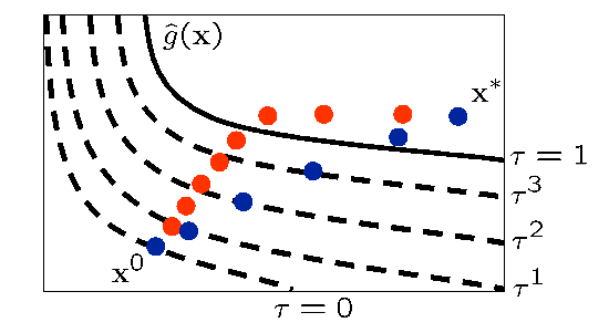
Fig. 83 Illustration of SBO iterates using surrogate (red) and relaxed(blue) constraints.
Fig. 83 illustrates the SBO algorithm on a two-dimensional problem with one inequality constraint starting from an infeasible point, \({\bf x}^0\). The minimizer of the problem is denoted as \({\bf x}^*\). Iterates generated using the surrogate constraints are shown in red, where feasibility is achieved first, and then progress is made toward the optimal point. The iterates generated using the relaxed constraints are shown in blue, where a balance of satisfying feasibility and optimality has been achieved, leading to fewer overall SBO iterations.
The behavior illustrated in Fig. 83 is an example where using the relaxed constraints over the surrogate constraints may improve the overall performance of the SBO algorithm by reducing the number of iterations performed. This improvement comes at the cost of solving the minimization subproblem in Eq. (252), which can be significant in some cases (i.e., when the cost of evaluating \({\bf {\hat g}}^k({\bf x})\) and \({\bf {\hat h}}^k({\bf x})\) is not negligible, such as with multifidelity or ROM surrogates). As shown in the numerical experiments involving the Barnes problem presented in [PerezRW04], the directions toward constraint violation reduction and objective function reduction may be in opposing directions. In such cases, the use of the relaxed constraints may result in an increase in the overall number of SBO iterations since feasibility must ultimately take precedence.