Bayesian Methods
This chapter covers various topics relating to Bayesian methods for inferring input parameter distributions for computer models, which is sometimes called “Bayesian calibration of computer models.” One common solution approach for Bayesian calibration involves Markov Chain Monte Carlo (MCMC) sampling.
Fundamentals, Proposal Densities, Pre-solve for MAP point, and Rosenbrock Example describe Bayesian fundamentals and then cover specialized approaches for accelerating the MCMC sampling process used within Bayesian inference.
Chain diagnostic metrics for analyzing the convergence of the MCMC chain are discussed in Chain Diagnostics.
Model Discrepancy describes ways of handling a discrepancy between the model estimate and the responses.
Experimental Design describes a way of determining the optimal experimental design to identify high-fidelity runs that can be used to best inform the calibration of a low-fidelity model. This is followed by a discussion of information-theoretic metrics in Information Theoretic Tools.
Finally, we conclude this chapter with a discussion of a new Bayesian approach in Measure-theoretic Stochastic Inverstion which does not use MCMC and relies on a measure-theoretic approach for stochastic inference instead of MCMC. In Dakota, the Bayesian methods called QUESO, GPMSA, and DREAM use Markov Chain Monte Carlo sampling. The Bayesian method called WASABI implements the measure-theoretic approach.
Fundamentals
Bayes Theorem [JB03], shown in (153), is used for performing inference. In particular, we derive the plausible parameter values based on the prior probability density and the data \(\boldsymbol{d}\). A typical case involves the use of a conservative prior notion of an uncertainty, which is then constrained to be consistent with the observational data. The result is the posterior parameter density of the parameters \(f_{\boldsymbol{\Theta |D}}\left( \boldsymbol{\theta |d} \right)\).
The likelihood function is used to describe how well a model’s predictions are supported by the data. The specific likelihood function currently used in Dakota is a Gaussian likelihood. This means that we assume the difference between the model quantity of interest (e.g. result from a computer simulation) and the experimental observations are Gaussian:
where \(\boldsymbol{\theta}\) are the parameters of a model quantity of interest \(q_i\) and \(\epsilon_i\) is a random variable that can encompass both measurement errors on \(d_i\) and modeling errors associated with the simulation quantity of interest \(q_i(\boldsymbol{\theta})\). If we have \(n\) observations, the probabilistic model defined by (154) results in a likelihood function for \(\boldsymbol{\theta}\) as shown in (155):
where the residual vector \(\boldsymbol{r}\) is defined from the differences between the model predictions and the corresponding observational data (i.e., \(r_i = q_i(\boldsymbol{\theta}) - d_i\) for \(i = 1,\dots,n\)), and \(\boldsymbol{\Sigma_d}\) is the covariance matrix of the Gaussian data uncertainties.
The negative log-likelihood is comprised of the misfit function
plus contributions from the leading normalization factor (\(\frac{n}{2}\log(2\pi)\) and \(\frac{1}{2}\log(|\boldsymbol{\Sigma_d}|)\)). It is evident that dropping \(\boldsymbol{\Sigma_d}\) from (156) (or equivalently, taking it to be the identity) results in the ordinary least squares (OLS) approach commonly used in deterministic calibration. For a fixed \(\boldsymbol{\Sigma_d}\) (no hyper-parameters in the calibration), minimizing the misfit function is equivalent to maximizing the likelihood function and results in a solution known as the maximum likelihood estimate (MLE), which will be the same as the OLS estimate when the residuals have no relative weighting (any multiple of identity in the data covariance matrix).
When incorporating the prior density, the maximum a posteriori probability (MAP) point is the solution that maximizes the posterior probability in (153). This point will differ from the MLE for cases of non-uniform prior probability.
In the sections to follow, we describe approaches for preconditioning the MCMC process by computing a locally-accurate proposal density and for jump-starting the MCMC process by pre-solving for the MAP point. Within Dakota, these are separate options: one can configure a run to use either or both, although it is generally advantageous to employ both when the necessary problem structure (i.e., derivative support) is present.
Proposal Densities
When derivatives of \(q(\theta)\) are readily available (e.g., from adjoint-capable simulations or from emulator models such as polynomial chaos, stochastic collocation, or Gaussian processes), we can form derivatives of the misfit function as
Neglecting the second term in (158) (a three-dimensional Hessian tensor dotted with the residual vector) results in the Gauss-Newton approximation to the misfit Hessian:
This approximation requires only gradients of the residuals, enabling its use in cases where models or model emulators only provide first-order derivative information. Since the second term in (158) includes the residual vector, it becomes less important as the residuals are driven toward zero. This makes the Gauss-Newton approximation a good approximation for solutions with small residuals. It also has the feature of being at least positive semi-definite, whereas the full misfit Hessian may be indefinite in general.
We are interested in preconditioning the MCMC sampling using an accurate local representation of the curvature of the posterior distribution, so we will define the MCMC proposal covariance to be the inverse of the Hessian of the negative log posterior. From (153) and simplifying notation to \(\pi_{\rm post}\) for the posterior and \(\pi_0\) for the prior, we have
A typical approach for defining a proposal density is to utilize a multivariate normal (MVN) distribution with mean centered at the current point in the chain and prescribed covariance. Thus, in the specific case of an MVN proposal, we will utilize the fact that the Hessian of the negative log prior for a normal prior distribution is just the inverse covariance:
For non-normal prior distributions, this is not true and, in the case of uniform or exponential priors, the Hessian of the negative log prior is in fact zero. However, as justified by the approximation of an MVN proposal distribution and the desire to improve the conditioning of the resulting Hessian, we will employ (161) for all prior distribution types.
From here, we follow [PMSG14] and decompose the prior covariance into its Cholesky factors, resulting in
where we again simplify notation to represent \(\nabla^2_{\boldsymbol{\theta}} \left[ -\log(\pi_{\rm post}(\boldsymbol{\theta})) \right]\) as \(\boldsymbol{H_{\rm nlpost}}\) and \(\nabla^2_{\boldsymbol{\theta}} M(\boldsymbol{\theta})\) as \(\boldsymbol{H_M}\). The inverse of this matrix is then
Note that the use of \(\boldsymbol{\Sigma}_{\boldsymbol{0}}^{-1}\) for the Hessian of the negative log prior in (161) provides some continuity between the default proposal covariance and the proposal covariance from Hessian-based preconditioning: if the contributions from \(\boldsymbol{H_M}\) are neglected, then \(\boldsymbol{H}_{\boldsymbol{\rm nlpost}}^{-1} = \boldsymbol{\Sigma_0}\), the default.
To address the indefiniteness of \(\boldsymbol{H_M}\) (or to reduce the cost for large-scale problems by using a low-rank Hessian approximation), we perform a symmetric eigenvalue decomposition of this prior-preconditioned misfit and truncate any eigenvalues below a prescribed tolerance, resulting in
for a matrix \(\boldsymbol{V}_r\) of truncated eigenvectors and a diagonal matrix of truncated eigenvalues \(\boldsymbol{\Lambda}_r = {\rm diag}(\lambda_1, \lambda_2, \dots, \lambda_r)\). We then apply the Sherman-Morrison-Woodbury formula to invert the sum of the decomposed matrix and identity as
for \(\boldsymbol{D}_r = {\rm diag}(\frac{\lambda_1}{\lambda_1+1}, \frac{\lambda_2}{\lambda_2+1}, \dots, \frac{\lambda_r}{\lambda_r+1})\). We now arrive at our final result for the covariance of the MVN proposal density:
Pre-solve for MAP point
When an emulator model is in use, it is inexpensive to pre-solve for the MAP point by finding the optimal values for \(\boldsymbol{\theta}\) that maximize the log posterior (minimize the negative log posterior):
This effectively eliminates the burn-in procedure for an MCMC chain where some initial portion of the Markov chain is discarded, as the MCMC chain can instead be initiated from a high probability starting point: the MAP solution. Further, a full Newton optimization solver can be used with the Hessian defined from (160), irregardless of whether the misfit Hessian is a full Hessian (residual values, gradients, and Hessians are available for (158)) or a Gauss-Newton Hessian (residual gradients are available for (159)). Note that, in this case, there is no MVN approximation as in Proposal Densities, so we will not employ (161). Rather, we employ the actual Hessians of the negative log priors for the prior distributions in use.
Rosenbrock Example
Defining two residuals as:
with \(\boldsymbol{d} = \boldsymbol{0}\) and \(\boldsymbol{\Sigma_d} = \text{diag}(\boldsymbol{.5})\), it is evident from (156) that \(M(\theta;d)\) is exactly the Rosenbrock function 1 with its well-known banana-shaped contours.
Assuming a uniform prior on \([-2,2]\), Fig. 70 and Fig. 71 show the effect of different proposal covariance components, with the default prior covariance (\(\boldsymbol{\Sigma_{MVN}} = \boldsymbol{\Sigma_0}\)) in Fig. 70 and a misfit Hessian-based proposal covariance (\(\boldsymbol{\Sigma_{MVN}} = \boldsymbol{H}_{\boldsymbol{M}}^{-1}\)) in Fig. 71.
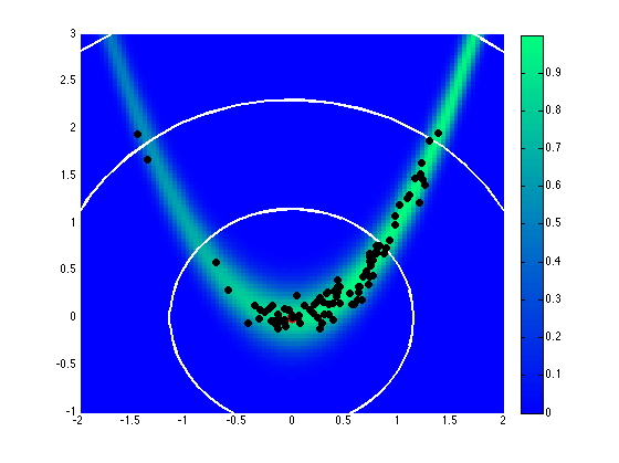
Fig. 70 Proposal covariance defined from uniform prior.
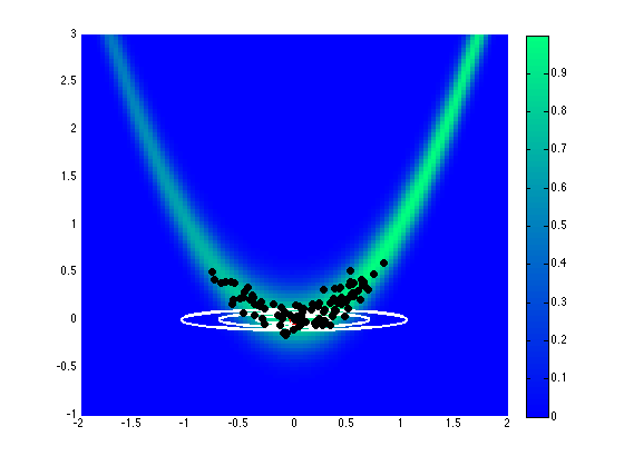
Fig. 71 Proposal covariance defined from uniform prior.
Rejection rates for 2000 MCMC samples were 73.4% for the former and 25.6% for the latter. Reducing the number of MCMC samples to 40, for purposes of assessing local proposal accuracy, results in a similar 72.5% rejection rate for prior-based proposal covariance and a reduced 17.5% rate for misfit Hessian-based proposal covariance. The prior-based proposal covariance only provides a global scaling and omits information on the structure of the likelihood; as a result, the rejection rates are relatively high for this problem and are not a strong function of location or chain length. The misfit Hessian-based proposal covariance, on the other hand, provides accurate local information on the structure of the likelihood, resulting in low rejection rates for samples in the vicinity of this Hessian update. Once the chain moves away from this vicinity, however, the misfit Hessian-based approach may become inaccurate and actually impede progress. This implies the need to regularly update a Hessian-based proposal covariance to sustain these MCMC improvements.
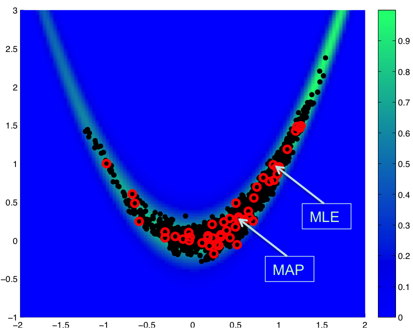
Fig. 72 Restarted chain
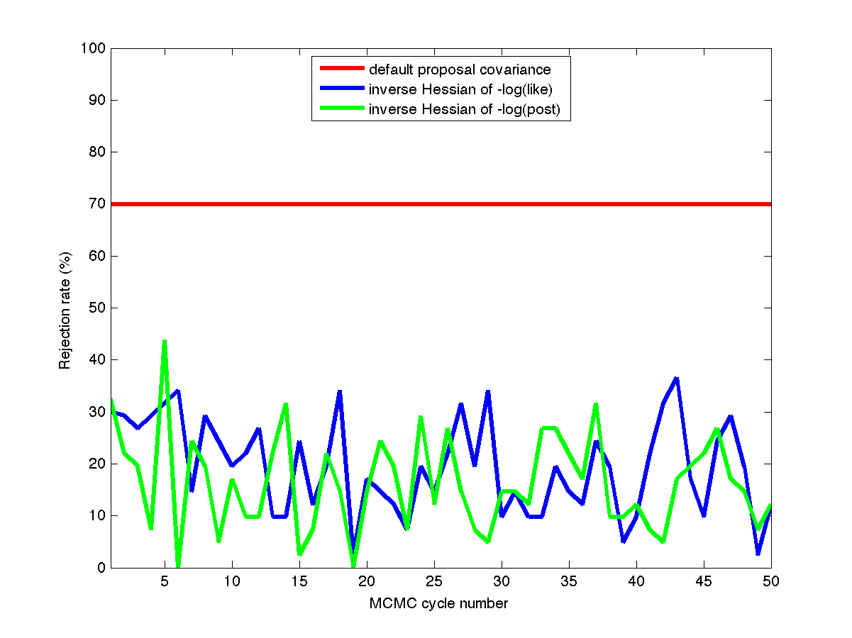
Fig. 73 Rejection rates
In Fig. 72, we show a result for a total of 2000 MCMC samples initiated from \((-1,1)\), where we restart the chain with an updated Hessian-based proposal covariance every 40 samples:
samples = 2000
proposal_updates = 50
This case uses a standard normal prior, resulting in differences in the MLE and MAP estimates, as shown in Fig. 72. Fig. 73 shows the history of rejection rates for each of the 50 chains for misfit Hessian-based proposals (\(\boldsymbol{\Sigma_{MVN}} = \boldsymbol{H}_{\boldsymbol{M}}^{-1}\)) and negative log posterior Hessian-based proposals (\(\boldsymbol{\Sigma_{MVN}} = \boldsymbol{H}_{\boldsymbol{\rm nlpost}}^{-1}\)) compared to the rejection rate for a single 2000-sample chain using prior-based proposal covariance (\(\boldsymbol{\Sigma_{MVN}} = \boldsymbol{\Sigma_0}\)).
A standard normal prior is not a strong prior in this case, and the posterior is likelihood dominated. This leads to similar performance from the two Hessian-based proposals, with average rejection rates of 70%, 19.5%, and 16.4% for prior-based, misfit Hessian-based, and posterior Hessian-based cases, respectively.
Chain Diagnostics
The implementation of a number of metrics for assessing the convergence
of the MCMC chain drawn during Bayesian calibration is undergoing active
development in Dakota. As of Dakota 6.10,
confidence_intervals is
the only diagnostic implemented.
Confidence Intervals
Suppose \(g\) is a function that represents some characteristic of the probability distribution \(\pi\) underlying the MCMC chain [FJ10], such as the mean or variance. Then under the standard assumptions of an MCMC chain, the true expected value of this function, \(\mathbb{E}_{\pi}g\) can be approximated by taking the mean over the \(n\) samples in the MCMC chain, denoted \(X = \{X_{1}, X_{2}, \ldots, X_{n} \}\),
The error in this approximation converges to zero, such that
Thus, in particular, we would like to estimate the variance of this error, \(\sigma_{g}^{2}\). Let \(\hat{\sigma}_{n}^{2}\) be a consistent estimator of the true variance \(\sigma_{g}^{2}\). Then
is an asymptotically valid interval estimator of \(\mathbb{E}_{\pi}g\), where \(t_{*}\) is a Student’s \(t\) quantile. In Dakota, confidence intervals are computed for the mean and variance of the parameters and of the responses, all confidence intervals are given at the 95th percentile, and \(\hat{\sigma}_{n}\) is calculated via non-overlapping batch means, or “batch means” for simplicity.
When batch means is used to calculate \(\hat{\sigma}_{n}\), the MCMC chain \(X\) is divided into blocks of equal size. Thus, we have \(a_{n}\) batches of size \(b_{n}\), and \(n = a_{n}b_{n}\). Then the batch means estimate of \(\sigma_{g}^{2}\) is given by
where \(\bar{g}_{k}\) is the expected value of \(g\) for batch \(k = 0, \ldots, a_{n}-1\),
It has been found that an appropriate batch size is \(b_{n} = \left \lfloor{\sqrt{n}}\right \rfloor\). Further discussion and comparison to alternate estimators of \(\sigma_{g}^{2}\) can be found in [FJ10].
Confidence intervals may be used as a chain diagnostic by setting fixed-width stopping rules [RKA18]. For example, if the width of one or more intervals is below some threshold value, that may indicate that enough samples have been drawn. Common choices for the threshold value include:
Fixed width: \(\epsilon\)
Relative magnitude: \(\epsilon \| \bar{g}_{n} \|\)
Relative standard deviation: \(\epsilon \| \hat{\sigma}_{n} \|\)
If the chosen threshold is exceeded, samples may need to be
increased. Sources [FJ10, RKA18] suggest increasing
the sample size by 10% and reevaluating the diagnostics for signs of
chain convergence.
If output is set to debug,
the sample mean and variance for each batch (for each parameter and response)
is output to the screen. The user can then analyze the convergence of these
batch means in order to deduce whether the MCMC chain has converged.
Model Discrepancy
Whether in a Bayesian setting or otherwise, the goal of model calibration is to minimize the difference between the observational data \(d_i\) and the corresponding model response \(q_i(\boldsymbol{\theta})\). That is, one seeks to minimize the misfit (156). For a given set of data, this formulation explicitly depends on model parameters that are to be adjusted and implicitly on conditions that may vary between experiments, such as temperature or pressure. These experimental conditions can be represented in Dakota by configuration variables, in which case (154) can be rewritten,
where \(x\) represents the configuration variables. Updated forms of the likelihood (155) and misfit (156) are easily obtained.
It is often the case that the calibrated model provides an insufficient fit to the experimental data. This is generally attributed to model form or structural error, and can be corrected to some extent with the use of a model discrepancy term. The seminal work in model discrepancy techniques, Kennedy and O’Hagan [KOHagan01], introduces an additive formulation
where \(\delta_i(x)\) represents the model discrepancy. For scalar responses, \(\delta_i\) depends only on the configuration variables, and one discrepancy model is calculated for each observable \(d_i\), \(i = 1, \ldots, n\), yielding \(\delta_1, \ldots, \delta_n\). For field responses in which the observational data and corresponding model responses are also functions of independent field coordinates such as time or space, (175) can be rewritten as
In this case, a single, global discrepancy model \(\delta\) is calculated over the entire field. The current model discrepancy implementation in Dakota has not been tested for cases in which scalar and field responses are mixed.
The Dakota implementation of model discrepancy for scalar responses also includes the calculation of prediction intervals for each prediction configuration \(x_{k,new}\). These intervals capture the uncertainty in the discrepancy approximation as well as the experimental uncertainty in the response functions. It is assumed that the uncertainties, representated by their respective variance values, are combined additively for each observable \(i\) such that
where \(\Sigma_{\delta,i}\) is the variance of the discrepancy function, and \(\sigma^2_{exp,i}\) is taken from the user-provided experimental variances. The experimental variance provided for parameter calibration may vary for the same observable from experiment to experiment, thus \(\sigma^{2}_{exp,i}\) is taken to be the maximum variance given for each observable. That is,
where \(\sigma^2_{i}(x_j)\) is the variance provided for the \(i^{th}\) observable \(d_i\), computed or measured with the configuration variable \(x_j\). When a Gaussian process discrepancy function is used, the variance is calculated according to (212). For polynomial discrepancy functions, the variance is given by (233).
It should be noted that a Gaussian process discrepancy function is used when the response is a field instead of a scalar; the option to use a polynomial discrepancy function has not yet been activated. The variance of the discrepancy function \(\Sigma_{\delta, i}\) is calculated according to (212). Future work includes extending this capability to include polynomial discrepancy formulations for field responses, as well as computation of prediction intervals which include experimental variance information.
Scalar Responses Example
For the purposes of illustrating the model discrepancy capability implemented in Dakota, consider the following example. Let the “truth” be given by
where \(t\) is the independent variable, \(x\) is the configuration parameter, and \(\theta^{*}\) is \(7.75\), the “true” value of the parameter \(\theta\). Let the “model” be given by
Again, \(t\) is the independent variable and \(x\) is the configuration parameter, and \(\theta\) now represents the model parameter to be calibrated. It is clear from the given formulas that the model is structurally different from the truth and will be inadequate.
The “experimental” data is produced by considering two configurations, \(x=10\) and \(x=15\). Data points are taken over the range \(t \in [1.2, 7.6]\) at intervals of length \(\Delta t = 0.4\). Normally distributed noise \(\epsilon_i\) is added such that
with \(i = 1, \ldots, 17\) and \(j = 1,2\). Performing a Bayesian update in Dakota yields a posterior distribution of \(\theta\) that is tightly peaked around the value \(\bar{\theta} = 7.9100\). Graphs of \(m(t, \bar{\theta}, 10)\) and \(m(t, \bar{\theta}, 15)\) are compared to \(y(t, 10)\) and \(y(t, 15)\), respectively, for \(t \in [1.2, 7.6]\) in Fig. 74, from which it is clear that the model insufficiently captures the given experimental data.
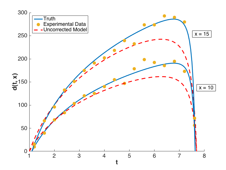
Fig. 74 Graphs of the uncorrected model output \(m(t,x)\), the truth \(y(t,x)\), and experimental data \(d(t,x)\) for configurations \(x = 10\) and \(x = 15\).
Following the Bayesian update, Dakota calculates the model discrepancy values
for the experimental data points, i.e. for \(i = 1, \ldots, 17\) and \(j = 1,2\). Dakota then approximates the model discrepancy functions \(\delta_1(x), \ldots \delta_{17}(x)\), and computes the responses and prediction intervals of the corrected model \(m_i(\bar{\theta}, x_{j,new}) + \delta_i(x_{j,new})\) for each prediction configuration. The prediction intervals have a radius of two times the standard deviation calculated with (177). The discrepancy function in this example was taken to be a Gaussian process with a quadratic trend, which is the default setting for the model discrepancy capability in Dakota.
The prediction configurations are taken to be \(x_{new} = 5, 5.5, \ldots, 20\). Examples of two corrected models are shown in Fig. 75. The substantial overlap in the measurement error bounds and the corrected model prediction intervals indicate that the corrected model is sufficiently accurate. This conclusion is supported by Fig. 78, in which the “truth” models for three prediction figurations are compared to the corrected model output. In each case, the truth falls within the prediction intervals.
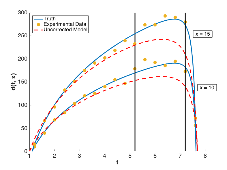
Fig. 75 Locations of the corrected models shown below.
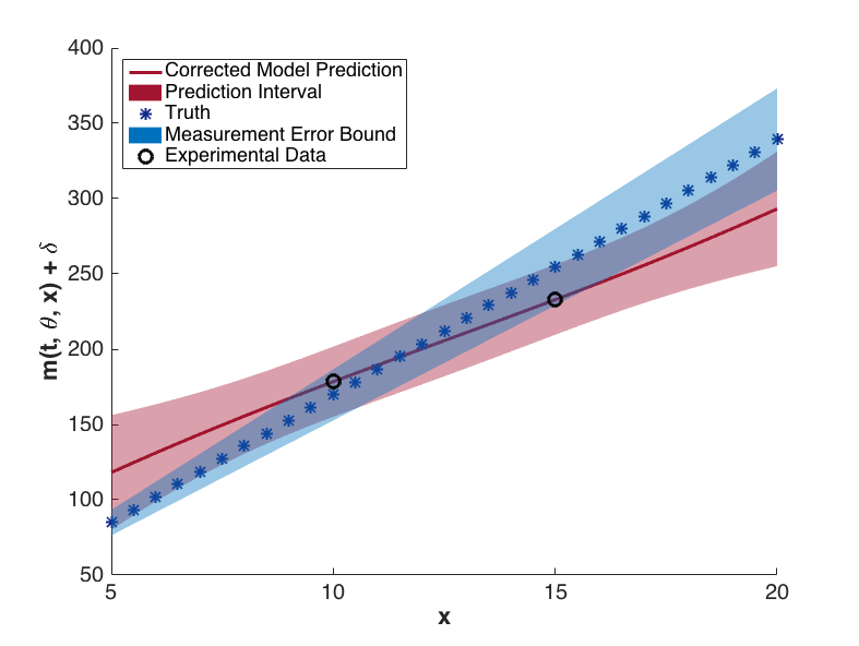
Fig. 76 Corrected model values with prediction intervals for t = 5.2
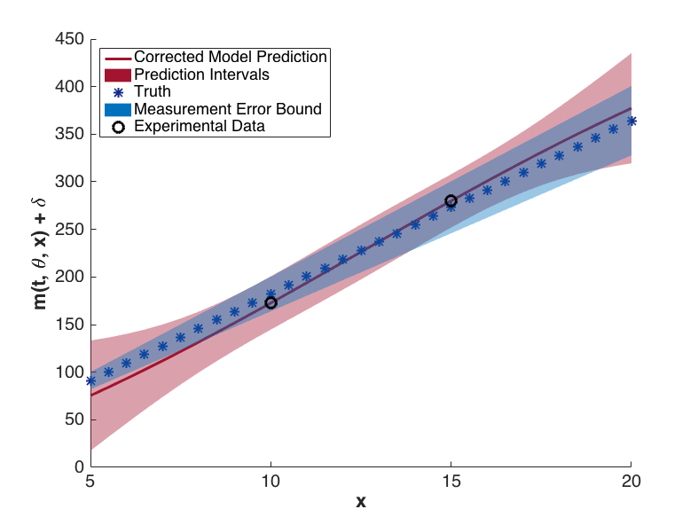
Fig. 77 Corrected model values with prediction intervals for t = 7.2
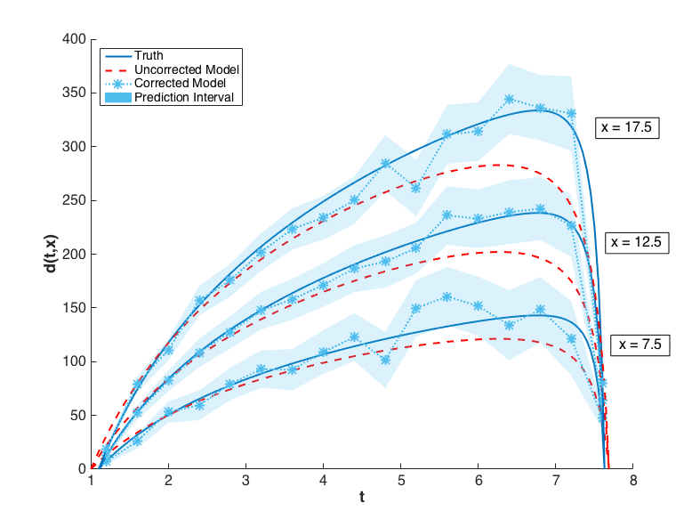
Fig. 78 The graphs of \(y(t,x)\) for \(x = 7.5, 12.5, 17.5\) are compared to the corrected model and its prediction intervals. The uncorrected model is also shown to illustrate its inadequacy.
Field Responses Example
To illustrate the model discrepancy capability for field responses, consider the stress-strain experimental data shown in Fig. 79. The configuration variable in this example represents temperature. Unlike the example discussed in the previous section, the domain of the independent variable (strain) differs from temperature to temperature, as do the shapes of the stress curves. This presents a challenge for the simulation model as well as the discrepancy model.
Let the “model” be given by
where \(t\) is the independent variable (strain) and \(x\) is the configuration parameter (temperature). Note that there are two parameters to be calibrated, \(\boldsymbol{\theta} = (\theta_{1}, \theta_{2})\).
The average and standard deviation of the experimental data at
temperatures \(x = 373.15\), \(x = 673.15\), and
\(x = 973.15\) are calculated and used as calibration data. The four
remaining temperatures will be used to evaluate the performance of the
corrected model. The calibration data and the resulting calibrated model
are shown in Figure 1.4. With experimental data,
the observations may not be taken at the same independent field
coordinates, so the keyword interpolate
can be used in the responses block of the Dakota input file.
The uncorrected model does not adequately capture the experimental data.
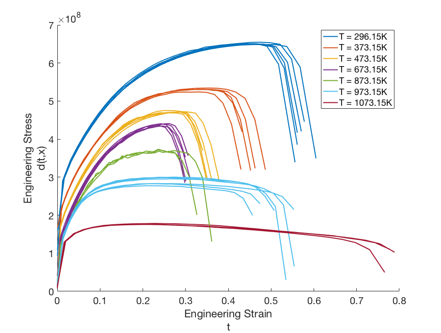
Fig. 79 Graphs of the experimental data \(d(t,x)\) for configurations (temperatures) ranging from \(x = 296.15K\) to \(x = 1073.15K\).
Following the Bayesian update, Dakota calculates the build points of the model discrepancy,
for each experimental data point. Dakota then approximates the global discrepancy function \(\delta(t, x)\) and computes the corrected model responses \(m(t_{i}, \boldsymbol{\theta}, x_{j, new}) + \delta(t_{i}, x_{j, new})\) and variance of the discrepancy model \(\sigma_{\delta, x_{j, new}}\) for each prediction configuration. The corrected model for the prediction configurations is shown in Fig. 80. The corrected model is able to capture the shape of the stress-strain curve quite well in all four cases; however, the point of failure is difficult to capture for the extrapolated temperatures. The difference in shape and point of failure between temperatures may also explain the large variance in the discrepancy model.
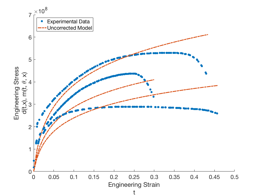
Fig. 80 Graphs of the calibration data \(d(t,x)\) and uncorrected calibrated model \(m(t, \boldsymbol{\theta}, x)\) for configurations (temperatures) \(x = 373.15K\), \(x = 673.15K\), and \(x = 973.15K\).
Experimental Design
Experimental design algorithms seek to add observational data that informs model parameters and reduces their uncertainties. Typically, the observational data \(\boldsymbol{d}\) used in the Bayesian update (153) is taken from physical experiments. However, it is also common to use the responses or output from a high-fidelity model as \(\boldsymbol{d}\) in the calibration of a low-fidelity model. Furthermore, this calibration can be done with a single Bayesian update or iteratively with the use of experimental design. The context of experimental design mandates that the high-fidelity model or physical experiment depend on design conditions or configurations, such as temperature or spatial location. After a preliminary Bayesian update using an initial set of high-fidelity (or experimental) data, the next “best” design points are determined and used in the high-fidelity model to augment \(\boldsymbol{d}\), which is used in subsequent Bayesian updates of the low-fidelity model parameters.
The question then becomes one of determining the meaning of “best.” In information theory, the mutual information is a measure of the reduction in the uncertainty of one random variable due to the knowledge of another [CT06]. Recast into the context of experimental design, the mutual information represents how much the proposed experiment and resulting observation would reduce the uncertainties in the model parameters. Therefore, given a set of experimental design conditions, that which maximizes the mutual information is the most desirable. This is the premise that motivates the Bayesian experimental design algorithm implemented in Dakota.
The initial set of high-fidelity data may be either user-specified or generated within Dakota by performing Latin Hypercube Sampling on the space of configuration variables specified in the input file. If Dakota-generated, the design variables will be run through the high-fidelity model specified by the user to produce the initial data set. Whether user-specified or Dakota-generated, this initial data is used in a Bayesian update of the low-fidelity model parameters.
It is important to note that the low-fidelity model depends on both parameters to be calibrated \(\boldsymbol{\theta}\) and the design conditions \(\boldsymbol{\xi}\). During Bayesian calibration, \(\boldsymbol{\xi}\) are not calibrated; they do, however, play an integral role in the calculation of the likelihood. Let us rewrite Bayes’ Rule as
making explicit the dependence of the data on the design conditions. As in Fundamentals, the difference between the high-fidelity and low-fidelity model responses is assumed to be Gaussian such that
where \(\boldsymbol{\xi}_{j}\) are the configuration specifications of the \(j\)th experiment. The experiments are considered to be independent, making the misfit
At the conclusion of the initial calibration, a set of candidate design conditions is proposed. As before, these may be either user-specified or generated within Dakota via Latin Hypercube Sampling of the design space. Among these candidates, we seek that which maximizes the mutual information,
where the mutual information is given by
The mutual information must, therefore, be computed for each candidate design point \(\boldsymbol{\xi}_{j}\). There are two \(k\)-nearest neighbor methods available in Dakota that can be used to approximate (189), both of which are derived in [KStogbauerG04]. Within Dakota, the posterior distribution \(f_{\boldsymbol{\Theta | D}}\left(\boldsymbol{\theta | d(\xi)}\right)\) is given by MCMC samples. From these, \(N\) samples are drawn and run through the low-fidelity model with \(\boldsymbol{\xi}_{j}\) fixed. This creates a matrix whose rows consist of the vector \(\boldsymbol{\theta}^{i}\) and the low-fidelity model responses \(\tilde{\boldsymbol{d}}(\boldsymbol{\theta}^{i}, \boldsymbol{\xi}_{j})\) for \(i = 1, \ldots, N\). These rows represent the joint distribution between the parameters and model responses. For each row \(X_{i}\), the distance to its \(k^{th}\)-nearest neighbor among the other rows is approximated \(\varepsilon_{i} = \| X_{i} - X_{k(i)} \|_{\infty}\). As noted in [LSWF16], \(k\) is often taken to be six. The treatment of the marginal distributions is where the two mutual information algorithms differ. In the first algorithm, the marginal distributions are considered by calculating \(n_{\boldsymbol{\theta},i}\), which is the number of parameter samples that lie within \(\varepsilon_{i}\) of \(\boldsymbol{\theta}^{i}\), and \(n_{\boldsymbol{d},i}\), which is the number of responses that lie within \(\varepsilon_{i}\) of \(\tilde{\boldsymbol{d}}(\boldsymbol{\theta}^{i}, \boldsymbol{\xi}_{j})\). The mutual information then is approximated as [KStogbauerG04]
where \(\psi(\cdot)\) is the digamma function.
In the second mutual information approximation method, \(X_{i}\) and all of its \(k\)-nearest neighbors such that \(\| X_{i} - X_{l} \|_{\infty} < \varepsilon_{i}\) are projected into the marginal subspaces for \(\boldsymbol{\theta}\) and \(\tilde{\boldsymbol{d}}\). The quantity \(\varepsilon_{\boldsymbol{\theta},i}\) is then defined as the radius of the \(l_{\infty}\)-ball containing all \(k+1\) projected values of \(\boldsymbol{\theta}_{l}\). Similarly, \(\varepsilon_{\boldsymbol{d},i}\) is defined as the radius of the \(l_{\infty}\)-ball containing all \(k+1\) projected values of \(\tilde{\boldsymbol{d}}(\boldsymbol{\theta}_{l}, \boldsymbol{\xi}_{j})\) [GVSG14]. In this version of the mutual information calculation, \(n_{\boldsymbol{\theta},i}\) is the number of parameter samples that lie within \(\varepsilon_{\boldsymbol{\theta},i}\) of \(\boldsymbol{\theta}^{i}\), and \(n_{\boldsymbol{d},i}\) is the number of responses that lie within \(\varepsilon_{\boldsymbol{d}, i}\) of \(\tilde{\boldsymbol{d}}(\boldsymbol{\theta}^{i}, \boldsymbol{\xi}_{j})\). The mutual information then is approximated as [KStogbauerG04]
By default, Dakota uses (190) to approximate the
mutual information. The user may decide to use
(191) by including the keyword ksg2 in the
Dakota input file.
Users also have the option of specifying
statistical noise in the low-fidelity model through the
simulation_variance keyword.
When this option is included in the
Dakota input file, a random “error” is added to the low-fidelity model
responses when the matrix \(X\) is built. This random error is
normally distributed, with variance equal to simulation_variance.
Once the optimal design \(\boldsymbol{\xi}^{*}\) is identified, it is run through the high-fidelity model to produce a new data point \(\boldsymbol{d}( \boldsymbol{\xi}^{*})\), which is added to the calibration data. Theoretically, the current posterior \(f_{\boldsymbol{\Theta | D}}\left(\boldsymbol{\theta | d(\xi)}\right)\) would become the prior in the new Bayesian update, and the misfit would compare the low-fidelity model output only to the new data point. However, as previously mentioned, we do not have the posterior distribution; we merely have a set of samples of it. Thus, each time the set of data is modified, the user-specified prior distribution is used and a full Bayesian update is performed from scratch. If none of the three stopping criteria is met, \(\boldsymbol{\xi}^{*}\) is removed from the set of candidate points, and the mutual information is approximated for those that remain using the newly updated parameters. These stopping criteria are:
the user-specified maximum number of high-fidelity model evaluations is reached (this does not include those needed to create the initial data set)
the relative change in mutual information from one iteration to the next is sufficiently small (less than \(5\%\))
the set of proposed candidate design conditions has been exhausted
If any one of these criteria is met, the algorithm is considered complete.
Batch Point Selection
The details of the experimental design algorithm above assume only one
optimal design point is being selected for each iteration of the
algorithm. The user may specify the number of optimal design points to
be concurrently selected by including the batch_size
in the input file. The optimality condition (188) is then replaced by
where \(\left\{ \boldsymbol{\xi}^{*} \right\} = \left\{ \boldsymbol{\xi}^{*}_{1},
\boldsymbol{\xi}_{2}^{*}, \ldots, \boldsymbol{\xi}_{s}^{*} \right\}\) is
the set of optimal designs, \(s\) being defined by batch_size.
If the set of design points from which the optimal designs are selected
is of size \(m\), finding \(\left\{ \boldsymbol{\xi}^{*} \right\}\) as
in (192) would require \(m!/(m-s)!\) mutual information
calculations, which may become quite costly. Dakota therefore implements a
greedy batch point selection algorithm in which the first optimal design,
is identified, and then used to find the second,
Generally, the \(i^{th}\) selected design will satisfy
The same mutual information calculation algorithms (190) and (191) described above are applied when calculating the conditional mutual information. The additional low-fidelity model information is appended to the responses portion of the matrix \(X\), and the calculation of \(\varepsilon_{i}\) or \(\varepsilon_{\boldsymbol{d}, i}\) as well as \(n_{\boldsymbol{d}, i}\) are adjusted accordingly.
Information Theoretic Tools
The notion of the entropy of a random variable was introduced by C.E. Shannon in 1948 [Sha48]. So named for its resemblance to the statistical mechanical entropy, the Shannon entropy (or simply the entropy), is characterized by the probability distribution of the random variable being investigated. For a random variable \(X \in \mathcal{X}\) with probability distribution function \(p\), the entropy \(h\) is given by
The entropy captures the average uncertainty in a random variable [CT06], and is therefore quite commonly used in predictive science. The entropy also provides the basis for other information measures, such as the relative entropy and the mutual information, both of which compare the information content between two random variables but have different purposes and interpretations.
The relative entropy provides a measure of the difference between two probability distributions. It is characterized by the Kullback-Leibler Divergence,
which can also be written as
where \(h(p,q)\) is the cross entropy of two distributions,
Because it is not symmetric (\(D_{KL} (p \| q) \neq D_{KL} (q \| p)\)), the Kullback-Leibler Divergence is sometimes referred to as a pseudo-metric. However, it is non-negative, and equals zero if and only if \(p = q\).
As in Experimental Design, the Kullback-Leibler Divergence is approximated with the \(k\)-nearest neighbor method advocated in [PerezC08]. Let the distributions \(p\) and \(q\) be represented by a collection of samples of size \(n\) and \(m\), respectively. For each sample \(x_{i}\) in \(p\), let \(\nu_{k}(i)\) be the distance to it’s \(k^{th}\)-nearest neighbor among the remaining samples of \(p\). Furthermore, let \(\rho_{k}(i)\) be the distance between \(x_{i}\) and its \(k^{th}\)-nearest neighbor among the samples of \(q\). If either of these distances is zero, the first non-zero neighbor distance is found, yielding a more general notation: \(\nu_{k_i}(i)\) and \(\rho_{l_i}(i)\), where \(k_{i}\) and \(l_{i}\) are the new neighbor counts and are greather than or equal to \(k\). Then
where \(\psi(\cdot)\) is the digamma function. In Dakota, \(k\) is taken to be six.
The Kullback-Leibler Divergence is used within Dakota to quantify the amount of information gained during Bayesian calibration,
If specified in the input file, the approximate value will be output to the screen at the end of the calibration.
In the presence of two (possibly multi-variate) random variables, the mutual information quantifies how much information they contain about each other. In this sense, it is a measure of the mutual dependence of two random variables. For continuous \(X\) and \(Y\),
where \(p(x,y)\) is the joint pdf of \(X\) and \(Y\), while \(p(x)\) and \(p(y)\) are the marginal pdfs of \(X\) and \(Y\), respectively. The mutual information is symmetric and non-negative, with zero indicating the independence of \(X\) and \(Y\). It is related to the Kullback-Leibler Divergence through the expression
The uses of the mutual information within Dakota have been noted in Experimental Design.
Measure-theoretic Stochastic Inversion
In this section we present an overview of a specific implementation of the measure-theoretic approach for solving a stochastic inverse problem that incorporates prior information and Bayes’ rule to define a unique solution. This approach differs from the standard Bayesian counterpart described in previous sections in that the posterior satisfies a consistency requirement with the model and the observed data. The material in this section is based on the foundational work in [BJW17, WWJ17]. A more thorough description of this consistent Bayesian approach and a comparison with the standard Bayesian approach can be found in [BJW17] and an extension to solve an optimal experimental design problem can be found in [WWJ17].
Let \(M(Y,\lambda)\) denote a deterministic model with solution \(Y(\lambda)\) that is an implicit function of model parameters \(\lambda\in\mathbf{\Lambda}\subset \mathbb{R}^n\). The set \(\mathbf{\Lambda}\) represents the largest physically meaningful domain of parameter values, and, for simplicity, we assume that \(\mathbf{\Lambda}\) is compact. We assume we are only concerned with computing a relatively small set of quantities of interest (QoI), \(\{Q_i(Y)\}_{i=1}^m\), where each \(Q_i\) is a real-valued functional dependent on the model solution \(Y\). Since \(Y\) is a function of parameters \(\lambda\), so are the QoI and we write \(Q_i(\lambda)\) to make this dependence explicit. Given a set of QoI, we define the QoI map \(Q(\lambda) := (Q_1(\lambda), \cdots, Q_m(\lambda))^\top:\mathbf{\Lambda}\to\mathbf{\mathcal{D}}\subset\mathbb{R}^m\) where \(\mathbf{\mathcal{D}}:= Q(\mathbf{\Lambda})\) denotes the range of the QoI map.
We assume \((\mathbf{\Lambda}, \mathcal{B}_{\mathbf{\Lambda}}, \mu_{\mathbf{\Lambda}})\) and \((\mathbf{\mathcal{D}}, \mathcal{B}_{\mathbf{\mathcal{D}}}, \mu_{\mathbf{\mathcal{D}}})\) are measure spaces and let \(\mathcal{B}_{\mathbf{\Lambda}}\) and \(\mathcal{B}_{\mathbf{\mathcal{D}}}\) denote the Borel \(\sigma\)-algebras inherited from the metric topologies on \(\mathbb{R}^n\) and \(\mathbb{R}^m\), respectively. We also assume that the QoI map \(Q\) is at least piecewise smooth implying that \(Q\) is a measurable map between the measurable spaces \((\mathbf{\Lambda}, \mathcal{B}_{\mathbf{\Lambda}})\) and \((\mathbf{\mathcal{D}}, \mathcal{B}_{\mathbf{\mathcal{D}}})\). For any \(A\in\mathcal{B}_{\mathbf{\mathcal{D}}}\), we then have
Furthermore, given any \(B\in\mathcal{B}_{\mathbf{\Lambda}}\),
although we note that in most cases \(B\neq Q^{-1}(Q(B))\) even when \(n=m\).
Finally, we assume that an observed probability measure, \(P_{\mathbf{\mathcal{D}}}^{\text{obs}}\), is given on \((\mathbf{\mathcal{D}},\mathcal{B}_{\mathbf{\mathcal{D}}})\), and the stochastic inverse problem seeks a probability measure \(P_\mathbf{\Lambda}\) such that the subsequent push-forward measure induced by the map, \(Q(\lambda)\), satisfies
for any \(A\in \mathcal{B}_{\mathbf{\mathcal{D}}}\).
This inverse problem may not have a unique solution, i.e., there may be multiple probability measures that have the proper push-forward measure. A unique solution may be obtained by imposing additional constraints or structure on the stochastic inverse problem. The approach we consider in this section incorporates prior information and Bayes rule to construct a unique solution to the stochastic inverse problem. The prior probability measure and the map induce a push-forward measure \(P_{\mathbf{\mathcal{D}}}^{Q(\text{prior})}\) on \(\mathbf{\mathcal{D}}\), which is defined for all \(A\in \mathcal{B}_{\mathbf{\mathcal{D}}}\),
We assume that all of the probability measures (prior, observed and push-forward of the prior) are absolutely continuous with respect to some reference measure and can be described in terms of a probability densities. We use \(\pi_{\mathbf{\Lambda}}^{\text{prior}}\), \(\pi_{\mathbf{\mathcal{D}}}^{\text{obs}}\) and \(\pi_{\mathbf{\mathcal{D}}}^{Q(\text{prior})}\) to denote the probability densities associated with \(P_{\mathbf{\Lambda}}^{\text{prior}}\), \(P_{\mathbf{\mathcal{D}}}^{\text{obs}}\) and \(P_{\mathbf{\mathcal{D}}}^{Q(\text{prior})}\) respectively. From [BJW17], the following posterior probability density, when interpreted through a disintegration theorem, solves the stochastic inverse problem:
One can immediately observe that if \(\pi_{\mathbf{\mathcal{D}}}^{Q(\text{prior})}= \pi_{\mathbf{\mathcal{D}}}^{\text{obs}}\), i.e., if the prior solves the stochastic inverse problem in the sense that the push-forward of the prior matches the observations, then the posterior will be equal to the prior. Approximating this posterior density requires an approximation of the push-forward of the prior, which is simply a forward propagation of uncertainty.
- 1
The two-dimensional Rosenbrock test function is defined as \(100 (x_2 - x_1^2)^2 + (1 - x_1)^2\)