Stochastic Expansion Methods
This chapter explores two approaches to forming stochastic expansions, the polynomial chaos expansion (PCE), which employs bases of multivariate orthogonal polynomials, and stochastic collocation (SC), which employs bases of multivariate interpolation polynomials. Both approaches capture the functional relationship between a set of output response metrics and a set of input random variables.
Orthogonal polynomials
Askey scheme
Table 16 shows the set of classical orthogonal polynomials which provide an optimal basis for different continuous probability distribution types. It is derived from the family of hypergeometric orthogonal polynomials known as the Askey scheme [AW85], for which the Hermite polynomials originally employed by Wiener [Wie38] are a subset. The optimality of these basis selections derives from their orthogonality with respect to weighting functions that correspond to the probability density functions (PDFs) of the continuous distributions when placed in a standard form. The density and weighting functions differ by a constant factor due to the requirement that the integral of the PDF over the support range is one.
Distribution |
Density function |
Polynomial |
Weight function |
Support range |
|---|---|---|---|---|
Normal |
\(\frac{1}{\sqrt{2\pi}} e^{\frac{-x^2}{2}}\) |
Hermite \(He_n(x)\) |
\(e^{\frac{-x^2}{2}}\) |
\([-\infty, \infty]\) |
Uniform |
\(\frac{1}{2}\) |
Legendre \(P_n(x)\) |
\(1\) |
\([-1,1]\) |
Beta |
\(\frac{(1-x)^{\alpha}(1+x)^{\beta}}{2^{\alpha+\beta+1}B(\alpha+1,\beta+1)}\) |
Jacobi \(P^{(\alpha,\beta)}_n(x)\) |
\((1-x)^{\alpha}(1+x)^{\beta}\) |
\([-1,1]\) |
Exponential |
\(e^{-x}\) |
Laguerre \(L_n(x)\) |
\(e^{-x}\) |
\([0, \infty]\) |
Gamma |
\(\frac{x^{\alpha} e^{-x}}{\Gamma(\alpha+1)}\) |
Generalized Laguerre \(L^{(\alpha)}_n(x)\) |
\(x^{\alpha} e^{-x}\) |
\([0, \infty]\) |
Note that Legendre is a special case of Jacobi for \(\alpha = \beta = 0\), Laguerre is a special case of generalized Laguerre for \(\alpha = 0\), \(\Gamma(a)\) is the Gamma function which extends the factorial function to continuous values, and \(B(a,b)\) is the Beta function defined as \(B(a,b) = \frac{\Gamma(a)\Gamma(b)}{\Gamma(a+b)}\). Some care is necessary when specifying the \(\alpha\) and \(\beta\) parameters for the Jacobi and generalized Laguerre polynomials since the orthogonal polynomial conventions [AS65] differ from the common statistical PDF conventions. The former conventions are used in Table 16.
Numerically generated orthogonal polynomials
If all random inputs can be described using independent normal, uniform, exponential, beta, and gamma distributions, then Askey polynomials can be directly applied. If correlation or other distribution types are present, then additional techniques are required. One solution is to employ nonlinear variable transformations such that an Askey basis can be applied in the transformed space. This can be effective as shown in [EWC08], but convergence rates are typically degraded. In addition, correlation coefficients are warped by the nonlinear transformation [DKL86], and simple expressions for these transformed correlation values are not always readily available. An alternative is to numerically generate the orthogonal polynomials (using Gauss-Wigert [Sim78], discretized Stieltjes [Gau04], Chebyshev [Gau04], or Gramm-Schmidt [WB06] approaches) and then compute their Gauss points and weights (using the Golub-Welsch [GW69] tridiagonal eigensolution). These solutions are optimal for given random variable sets having arbitrary probability density functions and eliminate the need to induce additional nonlinearity through variable transformations, but performing this process for general joint density functions with correlation is a topic of ongoing research (refer to “Transformations to uncorrelated standard variables” for additional details).
Interpolation polynomials
Interpolation polynomials may be either local or global and either value-based or gradient-enhanced: Lagrange (global value-based), Hermite (global gradient-enhanced), piecewise linear spline (local value-based), and piecewise cubic spline (local gradient-enhanced). Each of these combinations can be used within nodal or hierarchical interpolation formulations. The subsections that follow describe the one-dimensional interpolation polynomials for these cases and Section 1.4 describes their use for multivariate interpolation within the stochastic collocation algorithm.
Nodal interpolation
For value-based interpolation of a response function \(R\) in one dimension at an interpolation level \(l\) containing \(m^l\) points, the expression
reproduces the response values \(r(\xi_j)\) at the interpolation points and smoothly interpolates between these values at other points. As we refine the interpolation level, we increase the number of collocation points in the rule and the number of interpolated response values.
For the case of gradient-enhancement, interpolation of a one-dimensional function involves both type 1 and type 2 interpolation polynomials,
where the former interpolate a particular value while producing a zero gradient (\(i^{th}\) type 1 interpolant produces a value of 1 for the \(i^{th}\) collocation point, zero values for all other points, and zero gradients for all points) and the latter interpolate a particular gradient while producing a zero value (\(i^{th}\) type 2 interpolant produces a gradient of 1 for the \(i^{th}\) collocation point, zero gradients for all other points, and zero values for all points).
Global value-based
Lagrange polynomials interpolate a set of points in a single dimension using the functional form
where it is evident that \(L_j\) is 1 at \(\xi = \xi_j\), is 0 for each of the points \(\xi = \xi_k\), and has order \(m - 1\).
To improve numerical efficiency and stability, a barycentric Lagrange formulation [BT04, Hig04] is used. We define the barycentric weights \(w_j\) as
and we precompute them for a given interpolation point set \(\xi_j, j \in 1, ..., m\). Then, defining the quantity \(l(\xi)\) as
which will be computed for each new interpolated point \(\xi\), we can rewrite (72) as
where much of the computational work has been moved outside the summation. (77) is the first form of barycentric interpolation. Using an identity from the interpolation of unity (\(R(\xi) = 1\) and each \(r(\xi_j) = 1\) in (77)) to eliminate \(l(x)\), we arrive at the second form of the barycentric interpolation formula:
For both formulations, we reduce the computational effort for evaluating the interpolant from \(O(m^2)\) to \(O(m)\) operations per interpolated point, with the penalty of requiring additional care to avoid division by zero when \(\xi\) matches one of the \(\xi_j\). Relative to the first form, the second form has the additional advantage that common factors within the \(w_j\) can be canceled (possible for Clenshaw-Curtis and Newton-Cotes point sets, but not for general Gauss points), further reducing the computational requirements. Barycentric formulations can also be used for hierarchical interpolation with Lagrange interpolation polynomials, but they are not applicable to local spline or gradient-enhanced Hermite interpolants.
Global gradient-enhanced
Hermite interpolation polynomials (not to be confused with Hermite orthogonal polynomials shown in Table 16) interpolate both values and derivatives. In our case, we are interested in interpolating values and first derivatives, i.e, gradients. One-dimensional polynomials satisfying the interpolation constraints for general point sets are generated using divided differences as described in [Bur09a].
Local value-based
Linear spline basis polynomials define a “hat function,” which produces the value of one at its collocation point and decays linearly to zero at its nearest neighbors. In the case where its collocation point corresponds to a domain boundary, then the half interval that extends beyond the boundary is truncated.
For the case of non-equidistant closed points (e.g., Clenshaw-Curtis), the linear spline polynomials are defined as
For the case of equidistant closed points (i.e., Newton-Cotes), this can be simplified to
for \(h\) defining the half-interval \(\frac{b - a}{m - 1}\) of the hat function \(L_j\) over the range \(\xi \in [a, b]\). For the special case of \(m = 1\) point, \(L_1(\xi) = 1\) for \(\xi_1 = \frac{b+a}{2}\) in both cases above.
Local gradient-enhanced
Type 1 cubic spline interpolants are formulated as follows:
which produce the desired zero-one-zero property for left-center-right values and zero-zero-zero property for left-center-right gradients. Type 2 cubic spline interpolants are formulated as follows:
which produce the desired zero-zero-zero property for left-center-right values and zero-one-zero property for left-center-right gradients. For the special case of \(m = 1\) point over the range \(\xi \in [a, b]\), \(H_1^{(1)}(\xi) = 1\) and \(H_1^{(2)}(\xi) = \xi\) for \(\xi_1 = \frac{b+a}{2}\).
Hierarchical interpolation
In a hierarchical formulation, we reformulate the interpolation in terms of differences between interpolation levels:
where \(I^l(R)\) is as defined in (72) - (73) using the same local or global definitions for \(L_j(\xi)\), \(H_j^{(1)}(\xi)\), and \(H_j^{(2)}(\xi)\), and \(I^{l-1}(R)\) is evaluated as \(I^l(I^{l-1}(R))\), indicating reinterpolation of the lower level interpolant across the higher level point set [AA09, KW05].
Utilizing (72) - (73), we can represent this difference interpolant as
where \(I^{l-1}(R)(\xi_j)\) and \(\frac{dI^{l-1}(R)}{d\xi}(\xi_j)\) are the value and gradient, respectively, of the lower level interpolant evaluated at the higher level points. We then define hierarchical surpluses \({s, s^{(1)}, s^{(2)}}\) at a point \(\xi_j\) as the bracketed terms in (84). These surpluses can be interpreted as local interpolation error estimates since they capture the difference between the true values and the values predicted by the previous interpolant.
For the case where we use nested point sets among the interpolation levels, the interpolant differences for points contained in both sets are zero, allowing us to restrict the summations above to \(\sum_{j=1}^{m_{\Delta_l}}\) where we define the set \(\Xi_{\Delta_l} = \Xi_l \setminus \Xi_{l-1}\) that contains \(m_{\Delta_l} = m_l - m_{l-1}\) points. \(\Delta^l(R)\) then becomes
The original interpolant \(I^l(R)\) can be represented as a summation of these difference interpolants
Note
We will employ these hierarchical definitions within stochastic collocation on sparse grids in the main Hierarchical section.
Generalized Polynomial Chaos
The set of polynomials from Orthogonal polynomials and Numerically generated orthogonal polynomials are used as an orthogonal basis to approximate the functional form between the stochastic response output and each of its random inputs. The chaos expansion for a response \(R\) takes the form
where the random vector dimension is unbounded and each additional set of nested summations indicates an additional order of polynomials in the expansion. This expression can be simplified by replacing the order-based indexing with a term-based indexing
where there is a one-to-one correspondence between \(a_{i_1i_2...i_n}\) and \(\alpha_j\) and between \(B_n(\xi_{i_1},\xi_{i_2},...,\xi_{i_n})\) and \(\Psi_j(\boldsymbol{\xi})\). Each of the \(\Psi_j(\boldsymbol{\xi})\) are multivariate polynomials which involve products of the one-dimensional polynomials. For example, a multivariate Hermite polynomial \(B(\boldsymbol{\xi})\) of order \(n\) is defined from
which can be shown to be a product of one-dimensional Hermite polynomials involving an expansion term multi-index \(t_i^j\):
In the case of a mixed basis, the same multi-index definition is employed although the one-dimensional polynomials \(\psi_{t_i^j}\) are heterogeneous in type.
Expansion truncation and tailoring
In practice, one truncates the infinite expansion at a finite number of random variables and a finite expansion order
Traditionally, the polynomial chaos expansion includes a complete basis of polynomials up to a fixed total-order specification. That is, for an expansion of total order \(p\) involving \(n\) random variables, the expansion term multi-index defining the set of \(\Psi_j\) is constrained by
For example, the multidimensional basis polynomials for a second-order expansion over two random dimensions are
The total number of terms \(N_t\) in an expansion of total order \(p\) involving \(n\) random variables is given by
This traditional approach will be referred to as a “total-order expansion.”
An important alternative approach is to employ a “tensor-product expansion,” in which polynomial order bounds are applied on a per-dimension basis (no total-order bound is enforced) and all combinations of the one-dimensional polynomials are included. That is, the expansion term multi-index defining the set of \(\Psi_j\) is constrained by
where \(p_i\) is the polynomial order bound for the \(i^{th}\) dimension. In this case, the example basis for \(p = 2, n = 2\) is
and the total number of terms \(N_t\) is
It is apparent from (97) that the tensor-product expansion readily supports anisotropy in polynomial order for each dimension, since the polynomial order bounds for each dimension can be specified independently. It is also feasible to support anisotropy with total-order expansions, using a weighted multi-index constraint that is analogous to the one used for defining index sets in anisotropic sparse grids (see (118)). Finally, additional tailoring of the expansion form is used in the case of sparse grids through the use of a summation of anisotropic tensor expansions. In all cases, the specifics of the expansion are codified in the term multi-index, and subsequent machinery for estimating response values and statistics from the expansion can be performed in a manner that is agnostic to the specific expansion form.
Stochastic Collocation
The SC expansion is formed as a sum of a set of multidimensional interpolation polynomials, one polynomial per interpolated response quantity (one response value and potentially multiple response gradient components) per unique collocation point.
Value-Based Nodal
For value-based interpolation in multiple dimensions, a tensor-product of the one-dimensional polynomials (described in the Global value-based section and the Local value-based section) is used:
where \(\boldsymbol{i} = (m_1, m_2, \cdots, m_n)\) are the number of nodes used in the \(n\)-dimensional interpolation and \(\xi_{j_k}^{i_k}\) indicates the \(j^{th}\) point out of \(i\) possible collocation points in the \(k^{th}\) dimension. This can be simplified to
where \(N_p\) is the number of unique collocation points in the multidimensional grid. The multidimensional interpolation polynomials are defined as
where \(c_k^j\) is a collocation multi-index (similar to the expansion term multi-index in (90) that maps from the \(j^{th}\) unique collocation point to the corresponding multidimensional indices within the tensor grid, and we have dropped the superscript notation indicating the number of nodes in each dimension for simplicity. The tensor-product structure preserves the desired interpolation properties where the \(j^{th}\) multivariate interpolation polynomial assumes the value of 1 at the \(j^{th}\) point and assumes the value of 0 at all other points, thereby reproducing the response values at each of the collocation points and smoothly interpolating between these values at other unsampled points. When the one-dimensional interpolation polynomials are defined using a barycentric formulation as described in Global value-based section (i.e., (78)), additional efficiency in evaluating a tensor interpolant is achieved using the procedure in [Kli05], which amounts to a multi-dimensional extension to Horner’s rule for tensor-product polynomial evaluation.
Multivariate interpolation on Smolyak sparse grids involves a weighted sum of the tensor products in (98) with varying \(\boldsymbol{i}\) levels. For sparse interpolants based on nested quadrature rules (e.g., Clenshaw-Curtis, Gauss-Patterson, Genz-Keister), the interpolation property is preserved, but sparse interpolants based on non-nested rules may exhibit some interpolation error at the collocation points.
Gradient-Enhanced Nodal
For gradient-enhanced interpolation in multiple dimensions, we extend the formulation in (99) to use a tensor-product of the one-dimensional type 1 and type 2 polynomials (described in the Global gradient-enhanced section or the Local gradient-enhanced section):
The multidimensional type 1 basis polynomials are
where \(c_k^j\) is the same collocation multi-index described for (100) and the superscript notation indicating the number of nodes in each dimension has again been omitted. The multidimensional type 2 basis polynomials for the \(k^{th}\) gradient component are the same as the type 1 polynomials for each dimension except \(k\):
As for the value-based case, multivariate interpolation on Smolyak sparse grids involves a weighted sum of the tensor products in (101) with varying \(\boldsymbol{i}\) levels.
Hierarchical
In the case of multivariate hierarchical interpolation on nested grids, we are interested in tensor products of the one-dimensional difference interpolants described in Section 1.2.2, with
for value-based, and
for gradient-enhanced, where \(k\) indicates the gradient component being interpolated.
These difference interpolants are particularly useful within sparse grid interpolation, for which the \(\Delta^l\) can be employed directly within (113).
Spectral projection
The major practical difference between PCE and SC is that, in PCE, one must estimate the coefficients for known basis functions, whereas in SC, one must form the interpolants for known coefficients. PCE estimates its coefficients using either spectral projection or linear regression, where the former approach involves numerical integration based on random sampling, tensor-product quadrature, Smolyak sparse grids, or cubature methods. In SC, the multidimensional interpolants need to be formed over structured data sets, such as point sets from quadrature or sparse grids; approaches based on random sampling may not be used.
The spectral projection approach projects the response against each basis function using inner products and employs the polynomial orthogonality properties to extract each coefficient. Similar to a Galerkin projection, the residual error from the approximation is rendered orthogonal to the selected basis. From (91), taking the inner product of both sides with respect to \(\Psi_j\) and enforcing orthogonality yields:
where each inner product involves a multidimensional integral over the support range of the weighting function. In particular, \(\Omega = \Omega_1\otimes\dots\otimes\Omega_n\), with possibly unbounded intervals \(\Omega_j\subset\mathbb{R}\) and the tensor product form \(\varrho(\boldsymbol{\xi}) = \prod_{i=1}^n \varrho_i(\xi_i)\) of the joint probability density (weight) function. The denominator in (108) is the norm squared of the multivariate orthogonal polynomial, which can be computed analytically using the product of univariate norms squared
where the univariate inner products have simple closed form expressions for each polynomial in the Askey scheme [AS65] and are readily computed as part of the numerically-generated solution procedures described in Numerically generated orthogonal polynomials. Thus, the primary computational effort resides in evaluating the numerator, which is evaluated numerically using sampling, quadrature, cubature, or sparse grid approaches (and this numerical approximation leads to use of the term “pseudo-spectral” by some investigators).
Sampling
In the sampling approach, the integral evaluation is equivalent to computing the expectation (mean) of the response-basis function product (the numerator in (108)) for each term in the expansion when sampling within the density of the weighting function. This approach is only valid for PCE and since sampling does not provide any particular monomial coverage guarantee, it is common to combine this coefficient estimation approach with a total-order chaos expansion.
In computational practice, coefficient estimations based on sampling benefit from first estimating the response mean (the first PCE coefficient) and then removing the mean from the expectation evaluations for all subsequent coefficients. While this has no effect for quadrature/sparse grid methods (see following two sections) and little effect for fully-resolved sampling, it does have a small but noticeable beneficial effect for under-resolved sampling.
Tensor product quadrature
In quadrature-based approaches, the simplest general technique for approximating multidimensional integrals, as in (108), is to employ a tensor product of one-dimensional quadrature rules. Since there is little benefit to the use of nested quadrature rules in the tensor-product case 2, we choose Gaussian abscissas, i.e. the zeros of polynomials that are orthogonal with respect to a density function weighting, e.g. Gauss-Hermite, Gauss-Legendre, Gauss-Laguerre, generalized Gauss-Laguerre, Gauss-Jacobi, or numerically-generated Gauss rules.
We first introduce an index \(i\in\mathbb{N}_+\), \(i\ge1\). Then, for each value of \(i\), let \(\{\xi_1^i, \ldots,\xi_{m_i}^i\}\subset \Omega_i\) be a sequence of abscissas for quadrature on \(\Omega_i\). For \(f\in C^0(\Omega_i)\) and \(n=1\) we introduce a sequence of one-dimensional quadrature operators
with \(m_i\in\mathbb{N}\) given. When utilizing Gaussian quadrature, (110) integrates exactly all polynomials of degree less than \(2m_i -1\), for each \(i=1,\ldots, n\). Given an expansion order \(p\), the highest order coefficient evaluations (see (108)) can be assumed to involve integrands of at least polynomial order \(2p\) (\(\Psi\) of order \(p\) and \(R\) modeled to order \(p\)) in each dimension such that a minimal Gaussian quadrature order of \(p+1\) will be required to obtain good accuracy in these coefficients.
Now, in the multivariate case \(n>1\), for each \(f\in C^0(\Omega)\) and the multi-index \(\mathbf{i}=(i_1,\dots,i_n)\in\mathbb{N}_+^n\) we define the full tensor product quadrature formulas
Clearly, the above product needs \(\prod_{j=1}^n m_{i_j}\) function evaluations. Therefore, when the number of input random variables is small, full tensor product quadrature is a very effective numerical tool. On the other hand, approximations based on tensor product grids suffer from the curse of dimensionality since the number of collocation points in a tensor grid grows exponentially fast in the number of input random variables. For example, if (111) employs the same order for all random dimensions, \(m_{i_j} = m\), then (111) requires \(m^n\) function evaluations.
In [EB09], it is demonstrated that close synchronization of expansion form with the monomial resolution of a particular numerical integration technique can result in significant performance improvements. In particular, the traditional approach of exploying a total-order PCE (Eqs. (92) – (94)) neglects a significant portion of the monomial coverage for a tensor-product quadrature approach, and one should rather employ a tensor-product PCE (Eqs. (95) – (97)) to provide improved synchronization and more effective usage of the Gauss point evaluations. When the quadrature points are standard Gauss rules (i.e., no Clenshaw-Curtis, Gauss-Patterson, or Genz-Keister nested rules), it has been shown that tensor-product PCE and SC result in identical polynomial forms [CGI10], completely eliminating a performance gap that exists between total-order PCE and SC [EB09].
Smolyak sparse grids
If the number of random variables is moderately large, one should rather consider sparse tensor product spaces as first proposed by Smolyak [Smo63] and further investigated by Refs. [BNR00, FST05, GG98, NTW07, NTW08, XH05] that reduce dramatically the number of collocation points, while preserving a high level of accuracy.
Here we follow the notation and extend the description in Ref. [NTW07] to describe the Smolyak isotropic formulas \(\mathscr{A}({\rm w},n)\), where \({\rm w}\) is a level that is independent of dimension 3. The Smolyak formulas are just linear combinations of the product formulas in (111) with the following key property: only products with a relatively small number of points are used. With \(\mathscr{U}^0 = 0\) and for \(i \geq 1\) define
and we set \(|\mathbf{i}| = i_1+\cdots + i_n\). Then the isotropic Smolyak quadrature formula is given by
This form is preferred for use in forming hierarchical interpolants as described in Hierarchical interpolation and the main Hierarchical section. For nodal interpolants and polynomial chaos in sparse grids, the following equivalent form [WWozniakowski95] is often more convenient since it collapses repeated index sets
For each index set \(\mathbf{i}\) of levels, linear or nonlinear growth rules are used to define the corresponding one-dimensional quadrature orders. The following growth rules are employed for indices \(i \geq 1\), where closed and open refer to the inclusion and exclusion of the bounds within an interval, respectively:
Nonlinear growth rules are used for fully nested rules (e.g., Clenshaw-Curtis is closed fully nested and Gauss-Patterson is open fully nested), and linear growth rules are best for standard Gauss rules that take advantage of, at most, “weak” nesting (e.g., reuse of the center point).
Examples of isotropic sparse grids, constructed from the fully nested Clenshaw-Curtis abscissas and the weakly-nested Gaussian abscissas are shown in Fig. 64, where \(\Omega=[-1,1]^2\) and both Clenshaw-Curtis and Gauss-Legendre employ nonlinear growth 4 from (115) and (116), respectively. There, we consider a two-dimensional parameter space and a maximum level \({\rm w}=5\) (sparse grid \(\mathscr{A}(5,2)\)). To see the reduction in function evaluations with respect to full tensor product grids, we also include a plot of the corresponding Clenshaw-Curtis isotropic full tensor grid having the same maximum number of points in each direction, namely \(2^{\rm w}+1 = 33\).
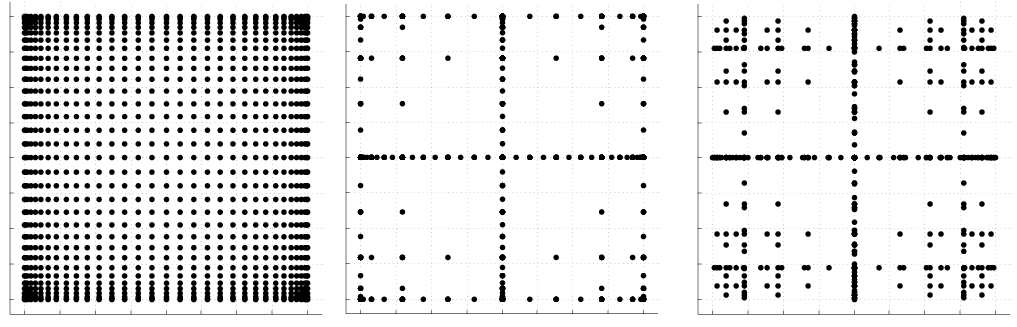
Fig. 64 Two-dimensional grid comparison with a tensor product grid using Clenshaw-Curtis points (left) and sparse grids \(\mathscr{A}(5,2)\) utilizing Clenshaw-Curtis (middle) and Gauss-Legendre (right) points with nonlinear growth.
In [EB09], it is demonstrated that the synchronization of total-order PCE with the monomial resolution of a sparse grid is imperfect, and that sparse grid SC consistently outperforms sparse grid PCE when employing the sparse grid to directly evaluate the integrals in (108). In our Dakota implementation, we depart from the use of sparse integration of total-order expansions, and instead employ a linear combination of tensor expansions [CEP12].
That is, we compute separate tensor polynomial chaos expansions for each of the underlying tensor quadrature grids (for which there is no synchronization issue) and then sum them using the Smolyak combinatorial coefficient (from (114) in the isotropic case). This improves accuracy, preserves the PCE/SC consistency property described in Tensor product quadrature, and also simplifies PCE for the case of anisotropic sparse grids described next.
For anisotropic Smolyak sparse grids, a dimension preference vector is used to emphasize important stochastic dimensions.
Given a mechanism for defining anisotropy, we can extend the definition of the sparse grid from that of (114) to weight the contributions of different index set components. First, the sparse grid index set constraint becomes
where \(\underline{\gamma}\) is the minimum of the dimension weights \(\gamma_k\), \(k\) = 1 to \(n\). The dimension weighting vector \(\mathbf{\gamma}\) amplifies the contribution of a particular dimension index within the constraint, and is therefore inversely related to the dimension preference (higher weighting produces lower index set levels). For the isotropic case of all \(\gamma_k = 1\), it is evident that you reproduce the isotropic index constraint \({\rm w}+1 \leq |\mathbf{i}| \leq {\rm w}+n\) (note the change from \(<\) to \(\leq\)). Second, the combinatorial coefficient for adding the contribution from each of these index sets is modified as described in [Bur09b].
Cubature
Cubature rules [Str71, Xiu08] are specifically optimized for multidimensional integration and are distinct from tensor-products and sparse grids in that they are not based on combinations of one-dimensional Gauss quadrature rules. They have the advantage of improved scalability to large numbers of random variables, but are restricted in integrand order and require homogeneous random variable sets (achieved via transformation). For example, optimal rules for integrands of 2, 3, and 5 and either Gaussian or uniform densities allow low-order polynomial chaos expansions (\(p=1\) or \(2\)) that are useful for global sensitivity analysis including main effects and, for \(p=2\), all two-way interactions.
Linear regression
Regression-based PCE approaches solve the linear system:
for a set of PCE coefficients \(\boldsymbol{\alpha}\) that best reproduce a set of response values \(\boldsymbol{R}\). The set of response values can be defined on an unstructured grid obtained from sampling within the density function of \(\boldsymbol{\xi}\) (point collocation [HWB07, Wal03]) or on a structured grid defined from uniform random sampling on the multi-index 5 of a tensor-product quadrature grid (probabilistic collocation [Tat95]), where the quadrature is of sufficient order to avoid sampling at roots of the basis polynomials 6. In either case, each row of the matrix \(\boldsymbol{\Psi}\) contains the \(N_t\) multivariate polynomial terms \(\Psi_j\) evaluated at a particular \(\boldsymbol{\xi}\) sample.
It is common to combine this coefficient estimation approach with a total-order chaos expansion in order to keep sampling requirements low. In this case, simulation requirements scale as \(\frac{r(n+p)!}{n!p!}\) (\(r\) is a collocation ratio with typical values \(0.1 \leq r \leq 2\)).
Additional regression equations can be obtained through the use of
derivative information (gradients and Hessians) from each collocation
point (see the
use_derivatives
keyword), which can aid in scaling with respect to the number of random variables,
particularly for adjoint-based derivative approaches.
Various methods can be employed to solve (119). The relative accuracy of each method is problem dependent. Traditionally, the most frequently used method has been least squares regression. However when \(\boldsymbol{\Psi}\) is under-determined, minimizing the residual with respect to the \(\ell_2\) norm typically produces poor solutions. Compressed sensing methods have been successfully used to address this limitation [BS11, DO11]. Such methods attempt to only identify the elements of the coefficient vector \(\boldsymbol{\alpha}\) with the largest magnitude and enforce as many elements as possible to be zero. Such solutions are often called sparse solutions. Dakota provides algorithms that solve the following formulations:
Basis Pursuit (BP) [CDS01]
(120)\[\boldsymbol{\alpha} = \text{arg min} \; \|\boldsymbol{\alpha}\|_{\ell_1}\quad \text{such that}\quad \boldsymbol{\Psi}\boldsymbol{\alpha} = \boldsymbol{R}\]The BP solution is obtained in Dakota, by transforming (120) to a linear program which is then solved using the primal-dual interior-point method [BV04, CDS01].
Basis Pursuit DeNoising (BPDN) [CDS01].
(121)\[\boldsymbol{\alpha} = \text{arg min}\; \|\boldsymbol{\alpha}\|_{\ell_1}\quad \text{such that}\quad \|\boldsymbol{\Psi}\boldsymbol{\alpha} - \boldsymbol{R}\|_{\ell_2} \le \varepsilon\]The BPDN solution is computed in Dakota by transforming (121) to a quadratic cone problem which is solved using the log-barrier Newton method [BV04, CDS01].
When the matrix \(\boldsymbol{\Psi}\) is not over-determined the BP and BPDN solvers used in Dakota will not return a solution. In such situations these methods simply return the least squares solution.
Orthogonal Matching Pursuit (OMP) [DMA97],
(122)\[\boldsymbol{\alpha} = \text{arg min}\; \|\boldsymbol{\alpha}\|_{\ell_0}\quad \text{such that}\quad \|\boldsymbol{\Psi}\boldsymbol{\alpha} - \boldsymbol{R}\|_{\ell_2} \le \varepsilon\]OMP is a heuristic method which greedily finds an approximation to (122). In contrast to the aforementioned techniques for solving BP and BPDN, which minimize an objective function, OMP constructs a sparse solution by iteratively building up an approximation of the solution vector \(\boldsymbol{\alpha}\). The vector is approximated as a linear combination of a subset of active columns of \(\boldsymbol{\Psi}\). The active set of columns is built column by column, in a greedy fashion, such that at each iteration the inactive column with the highest correlation (inner product) with the current residual is added.
Least Angle Regression (LARS) [EHJT04] and Least Absolute Shrinkage and Selection Operator (LASSO) [Tib96]
(123)\[ \boldsymbol{\alpha} = \text{arg min}\; \|\boldsymbol{\Psi}\boldsymbol{\alpha} - \boldsymbol{R}\|_{\ell_2}^2 \quad \text{such that}\|\boldsymbol{\alpha}\|_{\ell_1} \le \tau\]A greedy solution can be found to (123) using the LARS algorithm. Alternatively, with only a small modification, one can provide a rigorous solution to this global optimization problem, which we refer to as the LASSO solution. Such an approach is identical to the homotopy algorithm of Osborne et al [OPT00]. It is interesting to note that Efron [EHJT04] experimentally observed that the basic, faster LARS procedure is often identical to the LASSO solution.
The LARS algorithm is similar to OMP. LARS again maintains an active set of columns and again builds this set by adding the column with the largest correlation with the residual to the current residual. However, unlike OMP, LARS solves a penalized least squares problem at each step taking a step along an equiangular direction, that is, a direction having equal angles with the vectors in the active set. LARS and OMP do not allow a column (PCE basis) to leave the active set. However if this restriction is removed from LARS (it cannot be from OMP) the resulting algorithm can provably solve (123) and generates the LASSO solution.
Elastic net [ZH05]
(124)\[ \boldsymbol{\alpha} = \text{arg min}\; \|\boldsymbol{\Psi}\boldsymbol{\alpha} - \boldsymbol{R}\|_{\ell_2}^2 \quad \text{such that}\quad (1-\lambda)\|\boldsymbol{\alpha}\|_{\ell_1} + \lambda\|\boldsymbol{\alpha}\|_{\ell_2}^2 \le \tau\]The elastic net was developed to overcome some of the limitations of the LASSO formulation. Specifically: if the (\(M\times N\)) Vandermonde matrix \(\boldsymbol{\Psi}\) is over-determined (\(M>N\)), the LASSO selects at most \(N\) variables before it saturates, because of the nature of the convex optimization problem; if there is a group of variables among which the pairwise correlations are very high, then the LASSO tends to select only one variable from the group and does not care which one is selected; and finally if there are high correlations between predictors, it has been empirically observed that the prediction performance of the LASSO is dominated by ridge regression [Tib96]. Here we note that it is hard to estimate the \(\lambda\) penalty in practice and the aforementioned issues typically do not arise very often when solving (119). The elastic net formulation can be solved with a minor modification of the LARS algorithm.
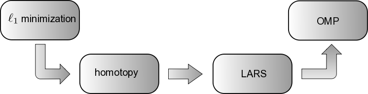
Fig. 65 Bridging provably convergent \(\ell_1\) minimization algorithms and greedy algorithms such as OMP. (1) Homotopy provably solves \(\ell_1\) minimization problems [EHJT04]. (2) LARS is obtained from homotopy by removing the sign constraint check. (3) OMP and LARS are similar in structure, the only difference being that OMP solves a least-squares problem at each iteration, whereas LARS solves a linearly penalized least-squares problem. Figure and caption based upon Figure 1 in [DT08].
OMP and LARS add a PCE basis one step at a time. If \(\boldsymbol{\alpha}\) contains only \(k\) non-zero terms then these methods will only take \(k\)-steps. The homotopy version of LARS also adds only basis at each step, however it can also remove bases, and thus can take more than \(k\) steps. For some problems, the LARS and homotopy solutions will coincide. Each step of these algorithm provides a possible estimation of the PCE coefficients. However, without knowledge of the target function, there is no easy way to estimate which coefficient vector is best. With some additional computational effort (which will likely be minor to the cost of obtaining model simulations), cross validation can be used to choose an appropriate coefficient vector.
Cross validation
Cross validation can be used to find a coefficient vector \(\boldsymbol{\alpha}\) that approximately minimizes \(\| \hat{f}(\mathbf{x})-f(\mathbf{x})\|_{L^2(\rho)}\), where \(f\) is the target function and \(\hat{f}\) is the PCE approximation using \(\boldsymbol{\alpha}\). Given training data \(\mathbf{X}\) and a set of algorithm parameters \(\boldsymbol{\beta}\) (which can be step number in an algorithm such as OMP, or PCE maximum degree), \(K\)-folds cross validation divides \(\mathbf{X}\) into \(K\) sets (folds) \(\mathbf{X}_k\), \(k=1,\ldots,K\) of equal size. A PCE \(\hat{f}^{-k}_{\boldsymbol{\beta}}(\mathbf{X})\), is built on the training data \(\mathbf{X}_{\mathrm{tr}}=\mathbf{X} \setminus \mathbf{X}_k\) with the \(k\)-th fold removed, using the tuning parameters \(\boldsymbol{\beta}\). The remaining data \(\mathbf{X}_k\) is then used to estimate the prediction error. The prediction error is typically approximated by \(e(\hat{f})=\lVert \hat{f}(\mathbf{x})-f(\mathbf{x})\rVert_{\ell_2}\), \(\mathbf{x}\in\mathbf{X}_{k}\) [HTF01]. This process is then repeated \(K\) times, removing a different fold from the training set each time.
The cross validation error is taken to be the average of the prediction errors for the \(K\)-experiments
We minimize \(CV(\hat{f}_{\boldsymbol{\beta}})\) as a surrogate for minimizing \(\| \hat{f}_{\boldsymbol{\beta}}(\mathbf{x})-f(\mathbf{x})\|_{L^2(\rho)}\) and choose the tuning parameters
to construct the final “best” PCE approximation of \(f\) that the training data can produce.
Iterative basis selection
When the coefficients of a PCE can be well approximated by a sparse vector, \(\ell_1\)-minimization is extremely effective at recovering the coefficients of that PCE. It is possible, however, to further increase the efficacy of \(\ell_1\)-minimization by leveraging realistic models of structural dependencies between the values and locations of the PCE coefficients. For example [BCDH10, DWB05, LD06] have successfully increased the performance of \(\ell_1\)-minimization when recovering wavelet coefficients that exhibit a tree-like structure. In this vein, we propose an algorithm for identifying the large coefficients of PC expansions that form a semi-connected subtree of the PCE coefficient tree.
The coefficients of polynomial chaos expansions often form a multi-dimensional tree. Given an ancestor basis term \(\phi_{\boldsymbol{\lambda}}\) of degree \(\left\lVert \boldsymbol{\lambda} \right\rVert_{1}\) we define the indices of its children as \(\boldsymbol{\lambda}+\mathbf{e}_k\), \(k=1,\ldots,d\), where \(\mathbf{e}_k=(0,\ldots,1,\ldots,0)\) is the unit vector co-directional with the \(k\)-th dimension.
An example of a typical PCE tree is depicted in Fig. 66. In this figure, as often in practice, the magnitude of the ancestors of a PCE coefficient is a reasonable indicator of the size of the child coefficient. In practice, some branches (connections) between levels of the tree may be missing. We refer to trees with missing branches as semi-connected trees.
In the following we present a method for estimating PCE coefficients that leverages the tree structure of PCE coefficients to increase the accuracy of coefficient estimates obtained by \(\ell_1\)-minimization.
![Tree structure of the coefficients of a two dimensional PCE with a total-degree basis of order 3. For clarity we only depict one connection per node, but in :math:`d` dimensions a node of a given degree :math:`p` will be a child of up to :math:`d` nodes of degree :math:`p-1`. For example, not only is the basis :math:`\boldsymbol{\phi}_{[1,1]}` a child of :math:`\boldsymbol{\phi}_{[1,0]}` (as depicted) but it is also a child of :math:`\boldsymbol{\phi}_{[0,1]}`](../../_images/pce-tree.png)
Fig. 66 Tree structure of the coefficients of a two dimensional PCE with a total-degree basis of order 3. For clarity we only depict one connection per node, but in \(d\) dimensions a node of a given degree \(p\) will be a child of up to \(d\) nodes of degree \(p-1\). For example, not only is the basis \(\boldsymbol{\phi}_{[1,1]}\) a child of \(\boldsymbol{\phi}_{[1,0]}\) (as depicted) but it is also a child of \(\boldsymbol{\phi}_{[0,1]}\)
Typically \(\ell_1\)-minimization is applied to an a priori chosen and fixed basis set \(\Lambda\). However the accuracy of coefficients obtained by \(\ell_1\)-minimization can be increased by adaptively selecting the PCE basis.
To select a basis for \(\ell_1\)-minimization we employ a four step iterative procedure involving restriction, expansion, identification and selection. The iterative basis selection procedure is outlined in Fig. 68. A graphical version of the algorithm is also presented in Fig. 67. The latter emphasizes the four stages of basis selection, that is restriction, growth, identification and selection. These four stages are also highlighted in Fig. 68 using the corresponding colors in Fig. 67.
To initiate the basis selection algorithm, we first define a basis set \(\Lambda^{(0)}\) and use \(\ell_1\)-minimization to identify the largest coefficients \(\boldsymbol{\alpha}^{(0)}\). The choice of \(\Lambda^{(0)}\) can sometimes affect the performance of the basis selection algorithm. We found a good choice to be \(\Lambda^{(0)}=\Lambda_{p,1}\), where \(p\) is the degree that gives \(\lvert\Lambda^d_{p,1}\rvert\) closest to \(10M\), i.e. \(\Lambda^d_{p,1} = \text{arg min}_{\Lambda^d_{p,1}\in\{\Lambda^d_{1,1},\Lambda^d_{2,1},\ldots\}}\lvert{\lvert\Lambda^d_{p,1}\rvert-10M}\rvert\). Given a basis \(\Lambda^{(k)}\) and corresponding coefficients \(\boldsymbol{\alpha}^{(k)}\) we reduce the basis to a set \(\Lambda^{(k)}_\varepsilon\) containing only the terms with non-zero coefficients. This restricted basis is then expanded \(T\) times using an algorithm which we will describe in Basis expansion. \(\ell_1\)-minimization is then applied to each of the expanded basis sets \(\Lambda^{(k,t)}\) for \(t=1,\dots, T\). Each time \(\ell_1\)-minimization is used, we employ cross validation to choose \(\varepsilon\). Therefore, at every basis set considered during the evolution of the algorithm we have a measure of the expected accuracy of the PCE coefficients. At each step in the algorithm we choose the basis set that results in the lowest cross validation error.
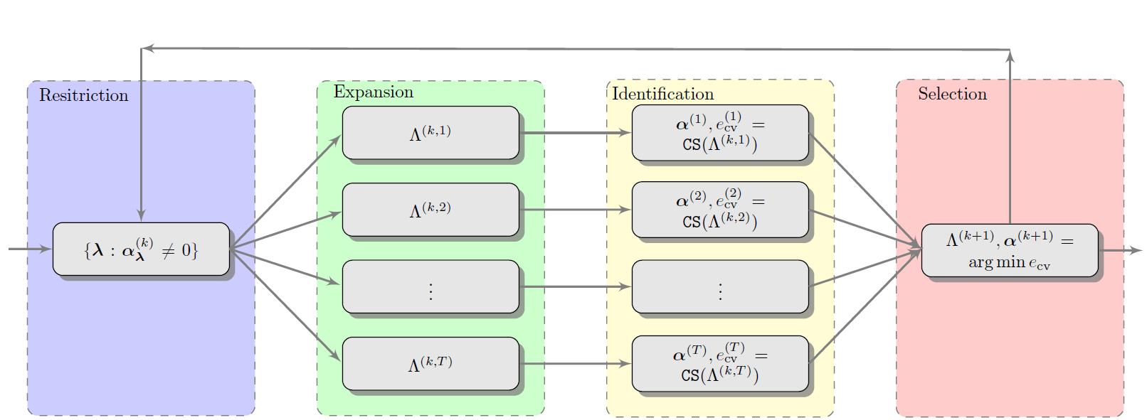
Fig. 67 Graphical depiction of the basis adaptation algorithm.
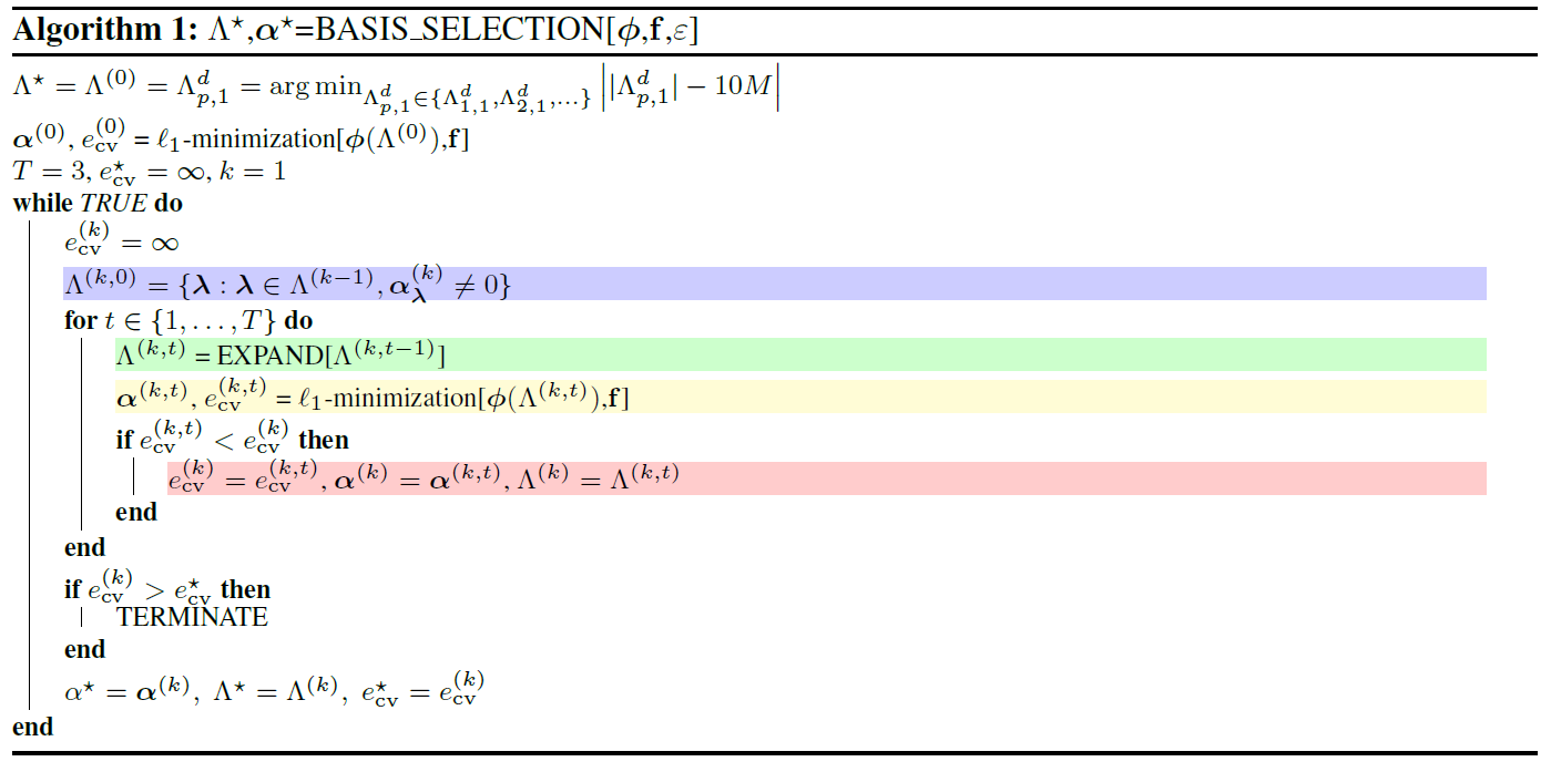
Fig. 68 Iterative basis selection procedure
Basis expansion
Define \(\{\boldsymbol{\lambda}+\mathbf{e}_j:1\le j\le d\}\) the forward neighborhood of an index \(\boldsymbol{\lambda}\) and similarly let \(\{\boldsymbol{\lambda}-\mathbf{e}_j:1\le j\le d\}\) denote the backward neighborhood. To expand a basis set \(\Lambda\) we must first find the forward neighbors \(\mathcal{F}=\{\boldsymbol{\lambda}+\mathbf{e}_j : \boldsymbol{\lambda}\in\Lambda, 1\le j\le d \}\) of all indices \(\boldsymbol{\lambda}\in\Lambda\). The expanded basis is then given by
where we have used the following admissibility criteria
to target PCE basis indices that are likely to have large PCE coefficients. A forward neighbor is admissible only if its backward neighbors exist in all dimensions. If the backward neighbors do not exist then \(\ell_1\)-minimization has previously identified that the coefficients of these backward neighbors are negligible.
The admissibility criterion is explained graphically in Fig. 69. In the left graphic, both children of the current index are admissible, because its backwards neighbors exist in every dimension. In the right graphic only the child in the vertical dimension is admissible, as not all parents of the horizontal child exist.
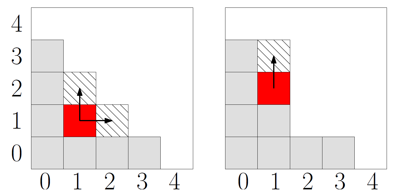
Fig. 69 Identification of the admissible indices of an index (red). The indices of the current basis \(\Lambda\) are gray and admissible indices are striped. A index is admissible only if its backwards neighbors exists in every dimension.
At the \(k\)-th iteration of Fig. 68, \(\ell_1\)-minimization is applied to \(\Lambda^{(k-1)}\) and used to identify the significant coefficients of the PCE and their corresponding basis terms \(\Lambda^{(k,0)}\). The set of non-zero coefficients \(\Lambda^{(k,0)}\) identified by \(\ell_1\)-minimization is then expanded.
The EXPAND routine
expands an index set by one polynomial degree, but sometimes it may be
necessary to expand the basis \(\Lambda^{(k)}\) more than once. 7
To generate these higher degree index sets EXPAND is applied
recursively to \(\Lambda^{(k,0)}\) up to a fixed number of \(T\)
times. Specifically, the following sets are generated
As the number of expansion steps \(T\) increases the number of terms in the expanded basis increases rapidly and degradation in the performance of \(\ell_1\)-minimization can result (this is similar to what happens when increasing the degree of a total degree basis). To avoid degradation of the solution, we use cross validation to choose the number of inner expansion steps \(t\in[1,T]\).
Orthogonal Least Interpolation
Orthogonal least interpolation (OLI) [NX12] enables the construction of interpolation polynomials based on arbitrarily located grids in arbitrary dimensions. The interpolation polynomials can be constructed using using orthogonal polynomials corresponding to the probability distribution function of the uncertain random variables.
The algorithm for constructing an OLI is split into three stages: (i) basis determination - transform the orthogonal basis into a polynomial space that is “amenable” for interpolation; (ii) coefficient determination - determine the interpolatory coefficients on the transformed basis elements; (iii) connection problem - translate the coefficients on the transformed basis to coefficients in the original orthogonal basis These three steps can be achieved by a sequence of LU and QR factorizations.
Orthogonal least interpolation is closesly related to the aforementioned regression methods, in that OLI can be used to build approximations of simulation models when computing structured simulation data, such as sparse grids or cubature nodes, is infeasiable. The interpolants produced by OLI have two additional important properties. Firstly, the orthogonal least interpolant is the lowest-degree polynomial that interpolates the data. Secondly, the least orthogonal interpolation space is monotonic. This second property means that the least interpolant can be extended to new data without the need to completely reconstructing the interpolant. The transformed interpolation basis can simply be extended to include the new necessary basis functions.
Analytic moments
Mean and covariance of polynomial chaos expansions are available in simple closed form:
where the norm squared of each multivariate polynomial is computed from (109). These expressions provide exact moments of the expansions, which converge under refinement to moments of the true response functions.
Similar expressions can be derived for stochastic collocation:
where we have simplified the expectation of Lagrange polynomials constructed at Gauss points and then integrated at these same Gauss points. For tensor grids and sparse grids with fully nested rules, these expectations leave only the weight corresponding to the point for which the interpolation value is one, such that the final equalities in (129) – (130) hold precisely. For sparse grids with non-nested rules, however, interpolation error exists at the collocation points, such that these final equalities hold only approximately. In this case, we have the choice of computing the moments based on sparse numerical integration or based on the moments of the (imperfect) sparse interpolant, where small differences may exist prior to numerical convergence. In Dakota, we employ the former approach; i.e., the right-most expressions in (129) – (130) are employed for all tensor and sparse cases irregardless of nesting. Skewness and kurtosis calculations as well as sensitivity derivations in the following sections are also based on this choice.
The expressions for skewness and (excess) kurtosis from direct numerical integration of the response function are as follows:
Local sensitivity analysis: derivatives with respect to expansion variables
Polynomial chaos expansions are easily differentiated with respect to the random variables [RNP+05]. First, using (91),
and then using (90),
where the univariate polynomial derivatives \(\frac{d\psi}{d\xi}\) have simple closed form expressions for each polynomial in the Askey scheme [AS65]. Finally, using the Jacobian of the (extended) Nataf variable transformation,
which simplifies to \(\frac{dR}{d\xi_i} \frac{d\xi_i}{dx_i}\) in the case of uncorrelated \(x_i\).
Similar expressions may be derived for stochastic collocation, starting from (99):
where the multidimensional interpolant \(\boldsymbol{L}_j\) is formed over either tensor-product quadrature points or a Smolyak sparse grid. For the former case, the derivative of the multidimensional interpolant \(\boldsymbol{L}_j\) involves differentiation of (100):
and for the latter case, the derivative involves a linear combination of these product rules, as dictated by the Smolyak recursion shown in (114). Finally, calculation of \(\frac{dR}{dx_i}\) involves the same Jacobian application shown in (135).
Global sensitivity analysis: variance-based decomposition
In addition to obtaining derivatives of stochastic expansions with respect to the random variables, it is possible to obtain variance-based sensitivity indices from the stochastic expansions. Variance-based sensitivity indices are explained in the Design of Experiments section. The concepts are summarized here as well. Variance-based decomposition is a global sensitivity method that summarizes how the uncertainty in model output can be apportioned to uncertainty in individual input variables. VBD uses two primary measures, the main effect sensitivity index \(S_{i}\) and the total effect index \(T_{i}\). These indices are also called the Sobol’ indices. The main effect sensitivity index corresponds to the fraction of the uncertainty in the output, \(Y\), that can be attributed to input \(x_{i}\) alone. The total effects index corresponds to the fraction of the uncertainty in the output, \(Y\), that can be attributed to input \(x_{i}\) and its interactions with other variables. The main effect sensitivity index compares the variance of the conditional expectation \(Var_{x_{i}}[E(Y|x_{i})]\) against the total variance \(Var(Y)\). Formulas for the indices are:
and
where \(Y=f({\bf x})\) and \({x_{-i}=(x_{1},...,x_{i-1},x_{i+1},...,x_{m})}\).
The calculation of \(S_{i}\) and \(T_{i}\) requires the evaluation of m-dimensional integrals which are typically approximated by Monte-Carlo sampling. However, in stochastic expansion methods, it is possible to obtain the sensitivity indices as analytic functions of the coefficients in the stochastic expansion. The derivation of these results is presented in [TIE10]. The sensitivity indices are printed as a default when running either polynomial chaos or stochastic collocation in Dakota. Note that in addition to the first-order main effects, \(S_{i}\), we are able to calculate the sensitivity indices for higher order interactions such as the two-way interaction \(S_{i,j}\).
Automated Refinement
Several approaches for refinement of stochastic expansions are currently supported, involving uniform or dimension-adaptive approaches to p- or h-refinement using structured (isotropic, anisotropic, or generalized) or unstructured grids. Specific combinations include:
uniform refinement with unbiased grids
p-refinement: isotropic global tensor/sparse grids (PCE, SC) and regression (PCE only) with global basis polynomials
h-refinement: isotropic global tensor/sparse grids with local basis polynomials (SC only)
dimension-adaptive refinement with biased grids
p-refinement: anisotropic global tensor/sparse grids with global basis polynomials using global sensitivity analysis (PCE, SC) or spectral decay rate estimation (PCE only)
h-refinement: anisotropic global tensor/sparse grids with local basis polynomials (SC only) using global sensitivity analysis
goal-oriented dimension-adaptive refinement with greedy adaptation
p-refinement: generalized sparse grids with global basis polynomials (PCE, SC)
h-refinement: generalized sparse grids with local basis polynomials (SC only)
Each involves incrementing the global grid using differing grid refinement criteria, synchronizing the stochastic expansion specifics for the updated grid, and then updating the statistics and computing convergence criteria. Future releases will support local h-refinement approaches that can replace or augment the global grids currently supported. The sub-sections that follow enumerate each of the first level bullets above.
Uniform refinement with unbiased grids
Uniform refinement involves ramping the resolution of a global
structured or unstructured grid in an unbiased manner and then refining
an expansion to synchronize with this increased grid resolution. In the
case of increasing the order of an isotropic tensor-product quadrature
grid or the level of an isotropic Smolyak sparse grid, a p-refinement
approach increases the order of the global basis polynomials
(See Orthogonal polynomials,
Global value-based,
and Global gradient-enhanced) in a synchronized manner
and an h-refinement approach reduces the approximation range of fixed
order local basis polynomials
(See Local value-based
and Local gradient-enhanced). And in the case of
uniform p-refinement with PCE regression, the collocation oversampling
ratio (see collocation_ratio)
is held fixed, such that an increment in isotropic expansion order is matched
with a corresponding increment
in the number of structured (probabilistic collocation) or unstructured
samples (point collocation) employed in the linear least squares solve.
For uniform refinement, anisotropic dimension preferences are not computed, and the only algorithmic requirements are:
With the usage of nested integration rules with restricted exponential growth, Dakota must ensure that a change in level results in a sufficient change in the grid; otherwise premature convergence could occur within the refinement process. If no change is initially detected, Dakota continues incrementing the order/level (without grid evaluation) until the number of grid points increases.
A convergence criterion is required. For uniform refinement, Dakota employs the \(L^2\) norm of the change in the response covariance matrix as a general-purpose convergence metric.
Dimension-adaptive refinement with biased grids
Dimension-adaptive refinement involves ramping the order of a tensor-product quadrature grid or the level of a Smolyak sparse grid anisotropically, that is, using a defined dimension preference. This dimension preference may be computed from local sensitivity analysis, global sensitivity analysis, a posteriori error estimation, or decay rate estimation. In the current release, we focus on global sensitivity analysis and decay rate estimation. In the former case, dimension preference is defined from total Sobol’ indices (see (139)) and is updated on every iteration of the adaptive refinement procedure, where higher variance attribution for a dimension indicates higher preference for that dimension. In the latter case, the spectral decay rates for the polynomial chaos coefficients are estimated using the available sets of univariate expansion terms (interaction terms are ignored). Given a set of scaled univariate coefficients (scaled to correspond to a normalized basis), the decay rate can be inferred using a technique analogous to Richardson extrapolation. The dimension preference is then defined from the inverse of the rate: slowly converging dimensions need greater refinement pressure. For both of these cases, the dimension preference vector supports anisotropic sparse grids based on a linear index-set constraint (see (118)) or anisotropic tensor grids (see (111)) with dimension order scaled proportionately to preference; for both grids, dimension refinement lower bound constraints are enforced to ensure that all previously evaluated points remain in new refined grids.
Given an anisotropic global grid, the expansion refinement proceeds as for the uniform case, in that the p-refinement approach increases the order of the global basis polynomials (see Orthogonal polynomials, Global value-based, and Global gradient-based) in a synchronized manner and an h-refinement approach reduces the approximation range of fixed order local basis polynomials (See Local value-based and Local gradient-enhanced). Also, the same grid change requirements and convergence criteria described for uniform refinement (See Uniform refinement with unbiased grids) are applied in this case.
Goal-oriented dimension-adaptive refinement with greedy adaptation
Relative to the uniform and dimension-adaptive refinement capabilities described previously, the generalized sparse grid algorithm [GG03] supports greater flexibility in the definition of sparse grid index sets and supports refinement controls based on general statistical quantities of interest (QOI). This algorithm was originally intended for adaptive numerical integration on a hypercube, but can be readily extended to the adaptive refinement of stochastic expansions using the following customizations:
In addition to hierarchical interpolants in SC, we employ independent polynomial chaos expansions for each active and accepted index set. Pushing and popping index sets then involves increments of tensor chaos expansions (as described in Smolyak sparse grids) along with corresponding increments to the Smolyak combinatorial coefficients.
Since we support bases for more than uniform distributions on a hypercube, we exploit rule nesting when possible (i.e., Gauss-Patterson for uniform or transformed uniform variables, and Genz-Keister for normal or transformed normal variables), but we do not require it. This implies a loss of some algorithmic simplifications in [GG03] that occur when grids are strictly hierarchical.
In the evaluation of the effect of a trial index set, the goal in [GG03] is numerical integration and the metric is the size of the increment induced by the trial set on the expectation of the function of interest. It is straightforward to instead measure the effect of a trial index set on response covariance, numerical probability, or other statistical QOI computed by post-processing the resulting PCE or SC expansion. By tying the refinement process more closely to the statistical QOI, the refinement process can become more efficient in achieving the desired analysis objectives.
Hierarchical increments in a variety of statistical QoI may be derived, starting from increments in response mean and covariance. The former is defined from computing the expectation of the difference interpolants in (104) - (105), and the latter is defined as:
Increments in standard deviation and reliability indices can
subsequently be defined, where care is taken to preserve numerical
precision through the square root operation (e.g., via Boost
sqrt1pm1()).
Given these customizations, the algorithmic steps can be summarized as:
Initialization: Starting from an initial isotropic or anisotropic reference grid (often the \(w=0\) grid corresponding to a single collocation point), accept the reference index sets as the old set and define active index sets using the admissible forward neighbors of all old index sets.
Trial set evaluation: Evaluate the tensor grid corresponding to each trial active index set, form the tensor polynomial chaos expansion or tensor interpolant corresponding to it, update the Smolyak combinatorial coefficients, and combine the trial expansion with the reference expansion. Perform necessary bookkeeping to allow efficient restoration of previously evaluated tensor expansions.
Trial set selection: Select the trial index set that induces the largest change in the statistical QOI, normalized by the cost of evaluating the trial index set (as indicated by the number of new collocation points in the trial grid). In our implementation, the statistical QOI is defined using an \(L^2\) norm of change in CDF/CCDF probability/reliability/response level mappings, when level mappings are present, or \(L^2\) norm of change in response covariance, when level mappings are not present.
Update sets: If the largest change induced by the trial sets exceeds a specified convergence tolerance, then promote the selected trial set from the active set to the old set and update the active sets with new admissible forward neighbors; return to step 2 and evaluate all trial sets with respect to the new reference point. If the convergence tolerance is satisfied, advance to step 5.
Finalization: Promote all remaining active sets to the old set, update the Smolyak combinatorial coefficients, and perform a final combination of tensor expansions to arrive at the final result for the statistical QOI.
Multifidelity methods
In a multifidelity uncertainty quantification approach employing stochastic expansions, we seek to utilize a predictive low-fidelity model to our advantage in reducing the number of high-fidelity model evaluations required to compute high-fidelity statistics to a particular precision. When a low-fidelity model captures useful trends of the high-fidelity model, then the model discrepancy may have either lower complexity, lower variance, or both, requiring less computational effort to resolve its functional form than that required for the original high-fidelity model [NE12].
To accomplish this goal, an expansion will first be formed for the model discrepancy (the difference between response results if additive correction or the ratio of results if multiplicative correction). These discrepancy functions are the same functions approximated in surrogate-based minimization. The exact discrepancy functions are
Approximating the high-fidelity response functions using approximations of these discrepancy functions then involves
where \(\hat{A}(\boldsymbol{\xi})\) and \(\hat{B}(\boldsymbol{\xi})\) are stochastic expansion approximations to the exact correction functions:
where \(\alpha_j\) and \(\beta_j\) are the spectral coefficients for a polynomial chaos expansion (evaluated via (108), for example) and \(a_j\) and \(b_j\) are the interpolation coefficients for stochastic collocation (values of the exact discrepancy evaluated at the collocation points).
Second, an expansion will be formed for the low fidelity surrogate model, where the intent is for the level of resolution to be higher than that required to resolve the discrepancy (\(P_{lo} \gg P_{hi}\) or \(N_{lo} \gg N_{hi}\); either enforced statically through order/level selections or automatically through adaptive refinement):
Then the two expansions are combined (added or multiplied) into a new expansion that approximates the high fidelity model, from which the final set of statistics are generated. For polynomial chaos expansions, this combination entails:
in the additive case, the high-fidelity expansion is formed by simply overlaying the expansion forms and adding the spectral coefficients that correspond to the same basis polynomials.
in the multiplicative case, the form of the high-fidelity expansion must first be defined to include all polynomial orders indicated by the products of each of the basis polynomials in the low fidelity and discrepancy expansions (most easily estimated from total-order, tensor, or sum of tensor expansions which involve simple order additions). Then the coefficients of this product expansion are computed as follows (shown generically for \(z = xy\) where \(x\), \(y\), and \(z\) are each expansions of arbitrary form):
(148)\[\begin{split}\begin{aligned} \sum_{k=0}^{P_z} z_k \Psi_k(\boldsymbol{\xi}) & = & \sum_{i=0}^{P_x} \sum_{j=0}^{P_y} x_i y_j \Psi_i(\boldsymbol{\xi}) \Psi_j(\boldsymbol{\xi}) \\ z_k & = & \frac{\sum_{i=0}^{P_x} \sum_{j=0}^{P_y} x_i y_j \langle \Psi_i \Psi_j \Psi_k \rangle}{\langle \Psi^2_k \rangle}\end{aligned}\end{split}\]where tensors of one-dimensional basis triple products \(\langle \psi_i \psi_j \psi_k \rangle\) are typically sparse and can be efficiently precomputed using one dimensional quadrature for fast lookup within the multidimensional triple products.
For stochastic collocation, the high-fidelity expansion generated from combining the low fidelity and discrepancy expansions retains the polynomial form of the low fidelity expansion, for which only the coefficients are updated in order to interpolate the sum or product values (and potentially their derivatives). Since we will typically need to produce values of a less resolved discrepancy expansion on a more resolved low fidelity grid to perform this combination, we utilize the discrepancy expansion rather than the original discrepancy function values for both interpolated and non-interpolated point values (and derivatives), in order to ensure consistency.
- 1
If joint distributions are known, then the Rosenblatt transformation is preferred.
- 2
Unless a refinement procedure is in use.
- 3
Other common formulations use a dimension-dependent level \(q\) where \(q \geq n\). We use \(w = q - n\), where \(w \geq 0\) for all \(n\).
- 4
We prefer linear growth for Gauss-Legendre, but employ nonlinear growth here for purposes of comparison.
- 5
Due to the discrete nature of index sampling, we enforce unique index samples by sorting and resampling as required.
- 6
Generally speaking, dimension quadrature order \(m_i\) greater than dimension expansion order \(p_i\).
- 7
The choice of \(T>1\) enables the basis selection algorithm to be applied to semi-connected tree structures as well as fully connected trees. Setting \(T>1\) allows us to prevent premature termination of the algorithm if most of the coefficients of the children of the current set \(\Lambda^{(k)}\) are small but the coefficients of the children’s children are not.