Models

Overview

Study Types describes the major categories of Dakota methods. A method evaluates or iterates on a model in order to map a set of variables into a set of responses. A model may involve a simple mapping with a single interface, or it may involve recursions using sub-methods and sub-models. These recursions permit “nesting,” “layering,” and “recasting” of software component building blocks to accomplish more sophisticated studies, such as surrogate-based optimization or optimization under uncertainty. In a nested relationship, a sub-method is executed using its sub-model for every evaluation of the nested model. In a layered relationship, on the other hand, sub-methods and sub-models are used only for periodic updates and verifications. And in a recast relationship, the input variable and output response definitions in a sub-model are reformulated in order to support new problem definitions. In each of these cases, the sub-model is of arbitrary type, such that model recursions can be chained together in as long of a sequence as needed (e.g., layered containing nested containing layered containing single as described in Surrogate-Based OUU (SBOUU)).

Fig. 29 displays the Model class hierarchy from the Dakota Developers Manual [ABC+23], with derived classes for single models, nested models, recast models, and two types of surrogate models: data fit and hierarchical/multifidelity. A third type of derived surrogate model supporting reduced-order models (ROM) is planned for future releases.

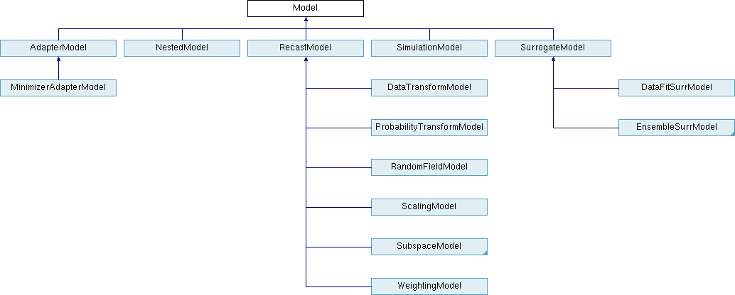
Fig. 29 The Dakota Model class hierarchy.

The following sections describe Single Models (a.k.a. Simulation Models), Recast Models, Surrogate Models (of various types), Nested Models, Random Field Models, and Active Subspace Models, in turn, followed by related educational screencasts on models. Finally, Advanced Model Recursions presents advanced examples demonstrating model recursions.

Single Models

The single (or simulation) model is the simplest model type. It uses a single interface to map variables to responses. There is no recursion in this case. See the single keyword for details on specifying single models.

Recast Models

Recast models do not appear in Dakota’s user input specification. Rather, they are used internally to transform the inputs and outputs of a sub-model in order to reformulate the problem posed to a method. Examples include variable and response scaling, transformations of uncertain variables and associated response derivatives to standardized random variables (see Reliability Methods and Stochastic Expansion Methods), multiobjective optimization, merit functions, and expected improvement/feasibility (see Derivative-Free Global Methods and Global Reliability Methods). Refer to the Dakota Developers Manual [ABC+23] for additional details on recasting.

Surrogate Models

Surrogate models are inexpensive approximate models intended to capture the salient features of an expensive high-fidelity model. They can be used to explore the variations in response quantities over regions of the parameter space, or they can serve as inexpensive stand-ins for optimization or uncertainty quantification studies (see, for example, Surrogate-Based Minimization). Dakota surrogate models are of one of three types: data fit, multifidelity, and reduced-order model. An overview and discussion of surrogate correction is provided here, with details following.

Note

There are video resources on Dakota surrogate models.

Overview of Surrogate Types

Data fitting methods involve construction of an approximation or surrogate model using data (response values, gradients, and Hessians) generated from the original truth model. Data fit methods can be further categorized into local, multipoint, and global approximation techniques, based on the number of points used in generating the data fit.

Warning

Known Issue: When using discrete variables, significant differences in data fit surrogate behavior have been observed across computing platforms in some cases. The cause has not been pinpointed. In addition, guidance on appropriate construction and use of surrogates is incomplete. In the meantime, users should be aware of the risk of inaccurate results when using surrogates with discrete variables.

Local methods involve response data from a single point in parameter space. Available local techniques currently include:

Taylor Series Expansion: This is a local first-order or second-order expansion centered at a single point in the parameter space.

Multipoint approximations involve response data from two or more points in parameter space, often involving the current and previous iterates of a minimization algorithm. Available techniques currently include:

TANA-3: This multipoint approximation uses a two-point exponential approximation [FRB90, XG98] built with response value and gradient information from the current and previous iterates.

Global methods, often referred to as response surface methods, involve many points spread over the parameter ranges of interest. These surface fitting methods work in conjunction with the sampling methods and design of experiments methods described in Sampling Methods and Design of Computer Experiments.

Polynomial Regression: First-order (linear), second-order (quadratic), and third-order (cubic) polynomial response surfaces computed using linear least squares regression methods. Note: there is currently no use of forward- or backward-stepping regression methods to eliminate unnecessary terms from the polynomial model.

An experimental least squares regression polynomial model was added in Dakota 6.12. The user may specify the basis functions in the polynomial through a total degree scheme.

Gaussian Process (GP) or Kriging Interpolation Dakota contains two supported implementations of Gaussian process, also known as Kriging [GW98], spatial interpolation. One of these resides in the Surfpack sub-package of Dakota, the other resides in Dakota itself. Both versions use the Gaussian correlation function with parameters that are selected by Maximum Likelihood Estimation (MLE). This correlation function results in a response surface that is \(C^\infty\)-continuous.

Note

Prior to Dakota 5.2, the Surfpack GP was referred to as the “Kriging” model and the Dakota version was labeled as the “Gaussian Process.” These terms are now used interchangeably. As of Dakota 5.2,the Surfpack GP is used by default. For now the user still has the option to select the Dakota GP, but the Dakota GP is deprecated and will be removed in a future release. A third experimental Gaussian process model was added in Dakota 6.12.

• Surfpack GP: Ill-conditioning due to a poorly spaced sample design is handled by discarding points that contribute the least unique information to the correlation matrix. Therefore, the points that are discarded are the ones that are easiest to predict. The resulting surface will exactly interpolate the data values at the retained points but is not guaranteed to interpolate the discarded points.

• Dakota GP: Ill-conditioning is handled by adding a jitter term or “nugget” to diagonal elements of the correlation matrix. When this happens, the Dakota GP may not exactly interpolate the data values.

• Experimental GP: This GP also contains a nugget parameter that may be fixed by the user or determined through MLE. When the nugget is greater than zero the mean of the GP is not forced to interpolate the response values.

Artificial Neural Networks: An implementation of the stochastic layered perceptron neural network developed by Prof. D. C. Zimmerman of the University of Houston [Zim96]. This neural network method is intended to have a lower training (fitting) cost than typical back-propagation neural networks.

Multivariate Adaptive Regression Splines (MARS): Software developed by Prof. J. H. Friedman of Stanford University [Fri91]. The MARS method creates a \(C^2\)-continuous patchwork of splines in the parameter space.

Radial Basis Functions (RBF): Radial basis functions are functions whose value typically depends on the distance from a center point, called the centroid. The surrogate model approximation is constructed as the weighted sum of individual radial basis functions.

Moving Least Squares (MLS): Moving Least Squares can be considered a more specialized version of linear regression models. MLS is a weighted least squares approach where the weighting is “moved” or recalculated for every new point where a prediction is desired. [Nea04]

Piecewise Decomposition Option for Global Surrogates: Typically, the previous regression techniques use all available sample points to approximate the underlying function anywhere in the domain. An alternative option is to use piecewise decomposition to locally approximate the function at some point using a few sample points from its neighborhood. This option currently supports Polynomial Regression, Gaussian Process (GP) Interpolation, and Radial Basis Functions (RBF) Regression. It requires a decomposition cell type (currently set to be Voronoi cells), an optional number of support layers of neighbors, and optional discontinuity detection parameters (jump/gradient).

In addition to data fit surrogates, Dakota supports multifidelity and reduced-order model approximations:

Multifidelity Surrogates: Multifidelity modeling involves the use of a low-fidelity physics-based model as a surrogate for the original high-fidelity model. The low-fidelity model typically involves a coarser mesh, looser convergence tolerances, reduced element order, or omitted physics. It is a separate model in its own right and does not require data from the high-fidelity model for construction. Rather, the primary need for high-fidelity evaluations is for defining correction functions that are applied to the low-fidelity results.

Reduced Order Models: A reduced-order model (ROM) is mathematically derived from a high-fidelity model using the technique of Galerkin projection. By computing a set of basis functions (e.g., eigenmodes, left singular vectors) that capture the principal dynamics of a system, the original high-order system can be projected to a much smaller system, of the size of the number of retained basis functions.

Correction Approaches

Each of the surrogate model types supports the use of correction factors that improve the local accuracy of the surrogate models. The correction factors force the surrogate models to match the true function values and possibly true function derivatives at the center point of each trust region. Currently, Dakota supports either zeroth-, first-, or second-order accurate correction methods, each of which can be applied using either an additive, multiplicative, or combined correction function. For each of these correction approaches, the correction is applied to the surrogate model and the corrected model is then interfaced with whatever algorithm is being employed. The default behavior is that no correction factor is applied.

The simplest correction approaches are those that enforce consistency in function values between the surrogate and original models at a single point in parameter space through use of a simple scalar offset or scaling applied to the surrogate model. First-order corrections such as the first-order multiplicative correction (also known as beta correction [CHGK93]) and the first-order additive correction [LN00] also enforce consistency in the gradients and provide a much more substantial correction capability that is sufficient for ensuring provable convergence in SBO algorithms. SBO convergence rates can be further accelerated through the use of second-order corrections which also enforce consistency in the Hessians [EGC04], where the second-order information may involve analytic, finite-difference, or quasi-Newton Hessians.

Correcting surrogate models with additive corrections involves

\[\hat{f_{hi_{\alpha}}}({\bf x}) = f_{lo}({\bf x}) + \alpha({\bf x}) \label{eq:correct_val_add}\]

where multifidelity notation has been adopted for clarity. For multiplicative approaches, corrections take the form

\[\hat{f_{hi_{\beta}}}({\bf x}) = f_{lo}({\bf x}) \beta({\bf x}) \label{eq:correct_val_mult}\]

where, for local corrections, \(\alpha({\bf x})\) and \(\beta({\bf x})\) are first or second-order Taylor series approximations to the exact correction functions:

\[ \begin{align}\begin{aligned}\alpha({\bf x}) & = A({\bf x_c}) + \nabla A({\bf x_c})^T ({\bf x} - {\bf x_c}) + \frac{1}{2} ({\bf x} - {\bf x_c})^T \nabla^2 A({\bf x_c}) ({\bf x} - {\bf x_c}) \label{eq:taylor_a}\\\beta({\bf x}) & = B({\bf x_c}) + \nabla B({\bf x_c})^T ({\bf x} - {\bf x_c}) + \frac{1}{2} ({\bf x} - {\bf x_c})^T \nabla^2 B({\bf x_c}) ({\bf x} - {\bf x_c}) \label{eq:taylor_b}\end{aligned}\end{align} \]

where the exact correction functions are

\[ \begin{align}\begin{aligned}A({\bf x}) & = f_{hi}({\bf x}) - f_{lo}({\bf x}) \label{eq:exact_A}\\B({\bf x}) & = \frac{f_{hi}({\bf x})}{f_{lo}({\bf x})} \label{eq:exact_B}\end{aligned}\end{align} \]

Refer to [EGC04] for additional details on the derivations.

A combination of additive and multiplicative corrections can provide for additional flexibility in minimizing the impact of the correction away from the trust region center. In other words, both additive and multiplicative corrections can satisfy local consistency, but through the combination, global accuracy can be addressed as well. This involves a convex combination of the additive and multiplicative corrections:

\[\hat{f_{hi_{\gamma}}}({\bf x}) = \gamma \hat{f_{hi_{\alpha}}}({\bf x}) + (1 - \gamma) \hat{f_{hi_{\beta}}}({\bf x}) \label{eq:combined_form}\]

where \(\gamma\) is calculated to satisfy an additional matching condition, such as matching values at the previous design iterate.

Data Fit Surrogate Models

A surrogate of the data fit type is a non-physics-based approximation typically involving interpolation or regression of a set of data generated from the original model. Data fit surrogates can be further characterized by the number of data points used in the fit, where a local approximation (e.g., first or second-order Taylor series) uses data from a single point, a multipoint approximation (e.g., two-point exponential approximations (TPEA) or two-point adaptive nonlinearity approximations (TANA)) uses a small number of data points often drawn from the previous iterates of a particular algorithm, and a global approximation (e.g., polynomial response surfaces, kriging/gaussian_process, neural networks, radial basis functions, splines) uses a set of data points distributed over the domain of interest, often generated using a design of computer experiments.

Dakota contains several types of surface fitting methods that can be used with optimization and uncertainty quantification methods and strategies such as surrogate-based optimization and optimization under uncertainty. These are: polynomial models (linear, quadratic, and cubic), first-order Taylor series expansion, kriging spatial interpolation, artificial neural networks, multivariate adaptive regression splines, radial basis functions, and moving least squares. With the exception of Taylor series methods, all of the above methods listed in the previous sentence are accessed in Dakota through the Surfpack library. All of these surface fitting methods can be applied to problems having an arbitrary number of design parameters. However, surface fitting methods usually are practical only for problems where there are a small number of parameters (e.g., a maximum of somewhere in the range of 30-50 design parameters). The mathematical models created by surface fitting methods have a variety of names in the engineering community. These include surrogate models, meta-models, approximation models, and response surfaces. For this manual, the terms surface fit model and surrogate model are used.

The data fitting methods in Dakota include software developed by Sandia researchers and by various researchers in the academic community.

Procedures for Surface Fitting

The surface fitting process consists of three steps: (1) selection of a set of design points, (2) evaluation of the true response quantities (e.g., from a user-supplied simulation code) at these design points, and (3) using the response data to solve for the unknown coefficients (e.g., polynomial coefficients, neural network weights, kriging correlation factors) in the surface fit model. In cases where there is more than one response quantity (e.g., an objective function plus one or more constraints), then a separate surface is built for each response quantity. Currently, most surface fit models are built using only 0\(^{\mathrm{th}}\)-order information (function values only), although extensions to using higher-order information (gradients and Hessians) are possible, and the Kriging model does allow construction for gradient data. Each surface fitting method employs a different numerical method for computing its internal coefficients. For example, the polynomial surface uses a least-squares approach that employs a singular value decomposition to compute the polynomial coefficients, whereas the kriging surface uses Maximum Likelihood Estimation to compute its correlation coefficients. More information on the numerical methods used in the surface fitting codes is provided in the Dakota Developers Manual [ABC+23].

The set of design points that is used to construct a surface fit model is generated using either the DDACE software package [TM] or the LHS software package [IS84]. These packages provide a variety of sampling methods including Monte Carlo (random) sampling, Latin hypercube sampling, orthogonal array sampling, central composite design sampling, and Box-Behnken sampling. See Design of Experiments for more information on these software packages. Optionally, the quality of a surrogate model can be assessed with surrogate metrics or diagnostics.

Taylor Series

The Taylor series model is purely a local approximation method. That is, it provides local trends in the vicinity of a single point in parameter space. The first-order Taylor series expansion is:

\[\hat{f}({\bf x}) \approx f({\bf x}_0) + \nabla_{\bf x} f({\bf x}_0)^T ({\bf x} - {\bf x}_0) \label{eq:taylor1}\]

and the second-order expansion is:

\[\hat{f}({\bf x}) \approx f({\bf x}_0) + \nabla_{\bf x} f({\bf x}_0)^T ({\bf x} - {\bf x}_0) + \frac{1}{2} ({\bf x} - {\bf x}_0)^T \nabla^2_{\bf x} f({\bf x}_0) ({\bf x} - {\bf x}_0) \label{eq:taylor2}\]

where \({\bf x}_0\) is the expansion point in \(n\)-dimensional parameter space and \(f({\bf x}_0),\) \(\nabla_{\bf x} f({\bf x}_0),\) and \(\nabla^2_{\bf x} f({\bf x}_0)\) are the computed response value, gradient, and Hessian at the expansion point, respectively. As dictated by the responses specification used in building the local surrogate, the gradient may be analytic or numerical and the Hessian may be analytic, numerical, or based on quasi-Newton secant updates.

In general, the Taylor series model is accurate only in the region of parameter space that is close to \({\bf x}_0\) . While the accuracy is limited, the first-order Taylor series model reproduces the correct value and gradient at the point \(\mathbf{x}_{0}\), and the second-order Taylor series model reproduces the correct value, gradient, and Hessian. This consistency is useful in provably-convergent surrogate-based optimization. The other surface fitting methods do not use gradient information directly in their models, and these methods rely on an external correction procedure in order to satisfy the consistency requirements of provably-convergent SBO.

Two Point Adaptive Nonlinearity Approximation

The TANA-3 method [XG98] is a multipoint approximation method based on the two point exponential approximation [FRB90]. This approach involves a Taylor series approximation in intermediate variables where the powers used for the intermediate variables are selected to match information at the current and previous expansion points. The form of the TANA model is:

\[\hat{f}({\bf x}) \approx f({\bf x}_2) + \sum_{i=1}^n \frac{\partial f}{\partial x_i}({\bf x}_2) \frac{x_{i,2}^{1-p_i}}{p_i} (x_i^{p_i} - x_{i,2}^{p_i}) + \frac{1}{2} \epsilon({\bf x}) \sum_{i=1}^n (x_i^{p_i} - x_{i,2}^{p_i})^2 \label{eq:tana_f}\]

where \(n\) is the number of variables and:

\[ \begin{align}\begin{aligned}p_i & = 1 + \ln \left[ \frac{\frac{\partial f}{\partial x_i}({\bf x}_1)} {\frac{\partial f}{\partial x_i}({\bf x}_2)} \right] \left/ \ln \left[ \frac{x_{i,1}}{x_{i,2}} \right] \right. \label{eq:tana_pi}\\\epsilon({\bf x}) & = \frac{H}{\sum_{i=1}^n (x_i^{p_i} - x_{i,1}^{p_i})^2 + \sum_{i=1}^n (x_i^{p_i} - x_{i,2}^{p_i})^2} \label{eq:tana_eps}\\H & = 2 \left[ f({\bf x}_1) - f({\bf x}_2) - \sum_{i=1}^n \frac{\partial f}{\partial x_i}({\bf x}_2) \frac{x_{i,2}^{1-p_i}}{p_i} (x_{i,1}^{p_i} - x_{i,2}^{p_i}) \right] \label{eq:tana_H}\end{aligned}\end{align} \]

and \({\bf x}_2\) and \({\bf x}_1\) are the current and previous expansion points. Prior to the availability of two expansion points, a first-order Taylor series is used.

Linear, Quadratic, and Cubic Polynomial Models

Linear, quadratic, and cubic polynomial models are available in Dakota. The form of the linear polynomial model is

\[\hat{f}(\mathbf{x}) \approx c_{0}+\sum_{i=1}^{n}c_{i}x_{i} \label{models:surf:equation01}\]

the form of the quadratic polynomial model is:

\[\hat{f}(\mathbf{x}) \approx c_{0}+\sum_{i=1}^{n}c_{i}x_{i} +\sum_{i=1}^{n}\sum_{j \ge i}^{n}c_{ij}x_{i}x_{j} \label{models:surf:equation02}\]

and the form of the cubic polynomial model is:

\[\hat{f}(\mathbf{x}) \approx c_{0}+\sum_{i=1}^{n}c_{i}x_{i} +\sum_{i=1}^{n}\sum_{j \ge i}^{n}c_{ij}x_{i}x_{j} +\sum_{i=1}^{n}\sum_{j \ge i}^{n}\sum_{k \ge j}^{n} c_{ijk}x_{i}x_{j}x_{k} \label{models:surf:equation03}\]

In all of the polynomial models, \(\hat{f}(\mathbf{x})\) is the response of the polynomial model; the \(x_{i},x_{j},x_{k}\) terms are the components of the \(n\)-dimensional design parameter values; the \(c_{0}\) , \(c_{i}\) , \(c_{ij}\) , \(c_{ijk}\) terms are the polynomial coefficients, and \(n\) is the number of design parameters. The number of coefficients, \(n_{c}\), depends on the order of polynomial model and the number of design parameters. For the linear polynomial:

\[n_{c_{linear}}=n+1 \label{models:surf:equation04}\]

for the quadratic polynomial:

\[n_{c_{quad}}=\frac{(n+1)(n+2)}{2} \label{models:surf:equation05}\]

and for the cubic polynomial:

\[n_{c_{cubic}}=\frac{(n^{3}+6 n^{2}+11 n+6)}{6} \label{models:surf:equation06}\]

There must be at least \(n_{c}\) data samples in order to form a fully determined linear system and solve for the polynomial coefficients. For discrete design variables, a further requirement for a well-posed problem is for the number of distinct values that each discrete variable can take must be greater than the order of polynomial model (by at least one level). For the special case involving anisotropy in which the degree can be specified differently per dimension, the number of values for each discrete variable needs to be greater than the corresponding order along the respective dimension. In Dakota, a least-squares approach involving a singular value decomposition numerical method is applied to solve the linear system.

The utility of the polynomial models stems from two sources: (1) over a small portion of the parameter space, a low-order polynomial model is often an accurate approximation to the true data trends, and (2) the least-squares procedure provides a surface fit that smooths out noise in the data. For this reason, the surrogate-based optimization approach often is successful when using polynomial models, particularly quadratic models. However, a polynomial surface fit may not be the best choice for modeling data trends over the entire parameter space, unless it is known a priori that the true data trends are close to linear, quadratic, or cubic. See [MM95] for more information on polynomial models.

This surrogate model supports the domain decomposition option.

An experimental polynomial model was added in Dakota 6.12 that is specified with experimental_polynomial. The user specifies the order of the polynomial through the required keyword basis_order according to a total degree rule.

Kriging/Gaussian-Process Spatial Interpolation Models

Dakota has three implementations of spatial interpolation models, two supported and one experimental. Of the supported versions, one is located in Dakota itself and the other in the Surfpack subpackage of Dakota which can be compiled in a standalone mode. These models are specified via gaussian_process dakota and gaussian_process surfpack.

Note

In Dakota releases prior to 5.2, the dakota version was referred to as the gaussian_process model while the surfpack version was referred to as the kriging model. As of Dakota 5.2, specifying only gaussian_process without qualification will default to the surfpack version in all contexts except Bayesian calibration. For now, both versions are supported but the dakota version is deprecated and likely to be removed in a future release. The two Gaussian process models are very similar; the differences between them are explained in more detail below.

The Kriging, also known as Gaussian process (GP), method uses techniques developed in the geostatistics and spatial statistics communities ([Cre91], [KO96]) to produce smooth surface fit models of the response values from a set of data points. The number of times the fitted surface is differentiable will depend on the correlation function that is used. Currently, the Gaussian correlation function is the only option for either version included in Dakota; this makes the GP model \(C^{\infty}\)-continuous. The form of the GP model is

\[\hat{f}(\underline{x}) \approx \underline{g}(\underline{x})^T\underline{\beta} + \underline{r}(\underline{x})^{T}\underline{\underline{R}}^{-1}(\underline{f}-\underline{\underline{G}}\ \underline{\beta}) \label{models:surf:equation08}\]

where \(\underline{x}\) is the current point in \(n\)-dimensional parameter space; \(\underline{g}(\underline{x})\) is the vector of trend basis functions evaluated at \(\underline{x}\); \(\underline{\beta}\) is a vector containing the generalized least squares estimates of the trend basis function coefficients; \(\underline{r}(\underline{x})\) is the correlation vector of terms between \(\underline{x}\) and the data points; \(\underline{\underline{R}}\) is the correlation matrix for all of the data points; \(\underline{f}\) is the vector of response values; and \(\underline{\underline{G}}\) is the matrix containing the trend basis functions evaluated at all data points. The terms in the correlation vector and matrix are computed using a Gaussian correlation function and are dependent on an \(n\)-dimensional vector of correlation parameters, \(\underline{\theta} = \{\theta_{1},\ldots,\theta_{n}\}^T\). By default, Dakota determines the value of \(\underline{\theta}\) using a Maximum Likelihood Estimation (MLE) procedure. However, the user can also opt to manually set them in the Surfpack Gaussian process model by specifying a vector of correlation lengths, \(\underline{l}=\{l_{1},\ldots,l_{n}\}^T\) where \(\theta_i=1/(2 l_i^2)\). This definition of correlation lengths makes their effect on the GP model’s behavior directly analogous to the role played by the standard deviation in a normal (a.k.a. Gaussian) distribution. In the Surfpack Gaussian process model, we used this analogy to define a small feasible region in which to search for correlation lengths. This region should (almost) always contain some correlation matrices that are well conditioned and some that are optimal, or at least near optimal. More details on Kriging/GP models may be found in [GW98].

Since a GP has a hyper-parametric error model, it can be used to model surfaces with slope discontinuities along with multiple local minima and maxima. GP interpolation is useful for both SBO and OUU, as well as for studying the global response value trends in the parameter space. This surface fitting method needs a minimum number of design points equal to the sum of the number of basis functions and the number of dimensions, \(n\), but it is recommended to use at least double this amount.

The GP model is guaranteed to pass through all of the response data values that are used to construct the model. Generally, this is a desirable feature. However, if there is considerable numerical noise in the response data, then a surface fitting method that provides some data smoothing (e.g., quadratic polynomial, MARS) may be a better choice for SBO and OUU applications. Another feature of the GP model is that the predicted response values, \(\hat{f}(\underline{x})\), decay to the trend function, \(\underline{g}(\underline{x})^T\underline{\beta}\), when \(\underline{x}\) is far from any of the data points from which the GP model was constructed (i.e., when the model is used for extrapolation).

As mentioned above, there are two primary Gaussian process models in Dakota, the surfpack version and the dakota version. More details on the Dakota GP model can be found in [McF08]. The differences between these models are as follows:

• Trend Function: The GP models incorporate a parametric trend function whose purpose is to capture large-scale variations. In both models, the trend function can be a constant, linear,or reduced quadratic (main effects only, no interaction terms) polynomial. This is specified by the keyword trend followed by one of constant, linear, or reduced_quadratic (in Dakota 5.0 and earlier, the reduced quadratic (second-order with no mixed terms) option for the dakota version was selected using the keyword, quadratic). The Surfpack GP model has the additional option of a full (including all interaction terms) quadratic polynomial that is specified with trend quadratic.

• Correlation Parameter Determination: Both of the primary GP models use a Maximum Likelihood Estimation (MLE) approach to find the optimal values of the hyper-parameters governing the mean and correlation functions. By default both models use the global optimization method called DIRECT, although they search regions with different extents. For the Dakota GP model, DIRECT is the only option. The Surfpack GP model has several options for hyperparameter optimization. These are specified by the optimization_method keyword followed by one of these strings:

  • 'global' which uses the default DIRECT optimizer,

  • 'local' which uses the CONMIN gradient-based optimizer,

  • 'sampling' which generates several random guesses and picks the candidate with greatest likelihood, and

  • 'none'

  The 'none' option and the initial iterate of the 'local' optimization default to the center, in log(correlation length) scale, of the small feasible region. However, these can also be user specified with the correlation_lengths keyword followed by a list of \(n\) real numbers. The total number of evaluations of the Surfpack GP model’s likelihood function can be controlled using the max_trials keyword followed by a positive integer. The 'global' optimization method tends to be the most robust, if slow to converge.

• Ill-conditioning. One of the major problems in determining the governing values for a Gaussian process or Kriging model is the fact that the correlation matrix can easily become ill-conditioned when there are too many input points close together. Since the predictions from the Gaussian process model involve inverting the correlation matrix, ill-conditioning can lead to poor predictive capability and should be avoided. The Surfpack GP model defines a small feasible search region for correlation lengths, which should (almost) always contain some well conditioned correlation matrices. In Dakota 5.1 and earlier, the Surfpack kriging model avoided ill-conditioning by explicitly excluding poorly conditioned \(\underline{\underline{R}}\) from consideration on the basis of their having a large (estimate of) condition number; this constraint acted to decrease the size of admissible correlation lengths. Note that a sufficiently bad sample design could require correlation lengths to be so short that any interpolatory Kriging/GP model would become inept at extrapolation and interpolation.

  The Dakota GP model has two features to overcome ill-conditioning. The first is that the algorithm will add a small amount of noise to the diagonal elements of the matrix (this is often referred to as a “nugget”) and sometimes this is enough to improve the conditioning. The second is that the user can specify to build the GP based only on a subset of points. The algorithm chooses an “optimal” subset of points (with respect to predictive capability on the remaining unchosen points) using a greedy heuristic. This option is specified with the keyword point_selection in the input file.

  As of Dakota 5.2, the Surfpack GP model has a similar capability. Points are not discarded prior to the construction of the model. Instead, within the maximum likelihood optimization loop, when the correlation matrix violates the explicit (estimate of) condition number constraint, a pivoted Cholesky factorization of the correlation matrix is performed. A bisection search is then used to efficiently find the last point for which the reordered correlation matrix is not too ill-conditioned. Subsequent reordered points are excluded from the GP/Kriging model for the current set of correlation lengths, i.e. they are not used to construct this GP model or compute its likelihood. When necessary, the Surfpack GP model will automatically decrease the order of the polynomial trend function. Once the maximum likelihood optimization has been completed, the subset of points that is retained will be the one associated with the most likely set of correlation lengths. Note that a matrix being ill-conditioned means that its rows or columns contain a significant amount of duplicate information. Since the points that were discarded were the ones that contained the least unique information, they should be the ones that are the easiest to predict and provide maximum improvement of the condition number. However, the Surfpack GP model is not guaranteed to exactly interpolate the discarded points. Warning: when two very nearby points are on opposite sides of a discontinuity, it is possible for one of them to be discarded by this approach.

  Note that a pivoted Cholesky factorization can be significantly slower than the highly optimized implementation of non-pivoted Cholesky factorization in typical LAPACK distributions. A consequence of this is that the Surfpack GP model can take significantly more time to build than the Dakota GP version. However, tests indicate that the Surfpack version will often be more accurate and/or require fewer evaluations of the true function than the Dakota analog. For this reason, the Surfpack version is the default option as of Dakota 5.2.

• Gradient Enhanced Kriging (GEK). As of Dakota 5.2, the use_derivatives keyword will cause the Surfpack GP model to be built from a combination of function value and gradient information. The Dakota GP model does not have this capability. Incorporating gradient information will only be beneficial if accurate and inexpensive derivative information is available, and the derivatives are not infinite or nearly so. Here “inexpensive” means that the cost of evaluating a function value plus gradient is comparable to the cost of evaluating only the function value, for example gradients computed by analytical, automatic differentiation, or continuous adjoint techniques. It is not cost effective to use derivatives computed by finite differences. In tests, GEK models built from finite difference derivatives were also significantly less accurate than those built from analytical derivatives. Note that GEK’s correlation matrix tends to have a significantly worse condition number than Kriging for the same sample design.

  This issue was addressed by using a pivoted Cholesky factorization of Kriging’s correlation matrix (which is a small sub-matrix within GEK’s correlation matrix) to rank points by how much unique information they contain. This reordering is then applied to whole points (the function value at a point immediately followed by gradient information at the same point) in GEK’s correlation matrix. A standard non-pivoted Cholesky is then applied to the reordered GEK correlation matrix and a bisection search is used to find the last equation that meets the constraint on the (estimate of) condition number. The cost of performing pivoted Cholesky on Kriging’s correlation matrix is usually negligible compared to the cost of the non-pivoted Cholesky factorization of GEK’s correlation matrix. In tests, it also resulted in more accurate GEK models than when pivoted Cholesky or whole-point-block pivoted Cholesky was performed on GEK’s correlation matrix.

This surrogate model supports the domain decomposition option.

The experimental Gaussian process model differs from the supported implementations in a few ways. First, at this time only local, gradient-based optimization methods for MLE are supported. The user may provide the num_restarts keyword to specify how many optimization runs from random initial iterates are performed. The appropriate number of starts to ensure that the global minimum is found is problem-dependent. When this keyword is omitted, the optimizer is run twenty times.

Second, build data for the surrogate is scaled to have zero mean and unit variance, and fixed bounds are imposed on the kernel hyperparameters. The type of scaling and bound specification will be made user-configrable in a future release.

Third, like the other GP implementations in Dakota the user may employ a polynomial trend function by supplying the trend keyword. Supported trend functions include constant, linear, reduced_quadratic and quadratic polynomials, the last of these being a full rather than reduced quadratic. Polynomial coefficients are determined alongside the kernel hyperparmeters through MLE.

Lastly, the use may specify a fixed non-negative value for the nugget parameter or may estimate it as part of the MLE procedure through the find_nugget keyword.

Artificial Neural Network (ANN) Models

The ANN surface fitting method in Dakota employs a stochastic layered perceptron (SLP) artificial neural network based on the direct training approach of Zimmerman [Zim96]. The SLP ANN method is designed to have a lower training cost than traditional ANNs. This is a useful feature for SBO and OUU where new ANNs are constructed many times during the optimization process (i.e., one ANN for each response function, and new ANNs for each optimization iteration). The form of the SLP ANN model is

\[\hat{f}(\mathbf{x}) \approx \tanh(\tanh((\mathbf{x A}_{0}+\theta_{0})\mathbf{A}_{1}+\theta_{1})) \label{models:surf:equation09}\]

where \(\mathbf{x}\) is the current point in \(n\)-dimensional parameter space, and the terms \(\mathbf{A}_{0},\theta_{0},\mathbf{A}_{1},\theta_{1}\) are the matrices and vectors that correspond to the neuron weights and offset values in the ANN model. These terms are computed during the ANN training process, and are analogous to the polynomial coefficients in a quadratic surface fit. A singular value decomposition method is used in the numerical methods that are employed to solve for the weights and offsets.

The SLP ANN is a non parametric surface fitting method. Thus, along with kriging and MARS, it can be used to model data trends that have slope discontinuities as well as multiple maxima and minima. However, unlike kriging, the ANN surface is not guaranteed to exactly match the response values of the data points from which it was constructed. This ANN can be used with SBO and OUU strategies. As with kriging, this ANN can be constructed from fewer than \(n_{c_{quad}}\) data points, however, it is a good rule of thumb to use at least \(n_{c_{quad}}\) data points when possible.

Multivariate Adaptive Regression Spline (MARS) Models

This surface fitting method uses multivariate adaptive regression splines from the MARS3.6 package [Fri91] developed at Stanford University.

The form of the MARS model is based on the following expression:

\[\hat{f}(\mathbf{x})=\sum_{m=1}^{M}a_{m}B_{m}(\mathbf{x}) \label{models:surf:equation10}\]

where the \(a_{m}\) are the coefficients of the truncated power basis functions \(B_{m}\), and \(M\) is the number of basis functions. The MARS software partitions the parameter space into subregions, and then applies forward and backward regression methods to create a local surface model in each subregion. The result is that each subregion contains its own basis functions and coefficients, and the subregions are joined together to produce a smooth, \(C^{2}\)-continuous surface model.

MARS is a nonparametric surface fitting method and can represent complex multimodal data trends. The regression component of MARS generates a surface model that is not guaranteed to pass through all of the response data values. Thus, like the quadratic polynomial model, it provides some smoothing of the data. The MARS reference material does not indicate the minimum number of data points that are needed to create a MARS surface model. However, in practice it has been found that at least \(n_{c_{quad}}\), and sometimes as many as 2 to 4 times \(n_{c_{quad}}\), data points are needed to keep the MARS software from terminating. Provided that sufficient data samples can be obtained, MARS surface models can be useful in SBO and OUU applications, as well as in the prediction of global trends throughout the parameter space.

Radial Basis Functions

Radial basis functions are functions whose value typically depends on the distance from a center point, called the centroid, \({\bf c}\). The surrogate model approximation is then built up as the sum of K weighted radial basis functions:

\[\hat{f}({\bf x})=\sum_{k=1}^{K}w_{k}\phi({\parallel {\bf x} - {\bf c_{k}} \parallel}) \label{models:surf:equation11}\]

where the \(\phi\) are the individual radial basis functions. These functions can be of any form, but often a Gaussian bell-shaped function or splines are used. Our implementation uses a Gaussian radial basis function. The weights are determined via a linear least squares solution approach. See [Orr96] for more details. This surrogate model supports the domain decomposition option.

Moving Least Squares

Moving Least Squares can be considered a more specialized version of linear regression models. In linear regression, one usually attempts to minimize the sum of the squared residuals, where the residual is defined as the difference between the surrogate model and the true model at a fixed number of points. In weighted least squares, the residual terms are weighted so the determination of the optimal coefficients governing the polynomial regression function, denoted by \(\hat{f}({\bf x})\), are obtained by minimizing the weighted sum of squares at N data points:

\[\sum_{n=1}^{N}w_{n}({\parallel \hat{f}({\bf x_{n}})-f({\bf x_{n}})\parallel}) \label{models:surf:equation12}\]

Moving least squares is a further generalization of weighted least squares where the weighting is “moved” or recalculated for every new point where a prediction is desired. [Nea04] The implementation of moving least squares is still under development. We have found that it works well in trust region methods where the surrogate model is constructed in a constrained region over a few points. It does not appear to be working as well globally, at least at this point in time.

Piecewise Decomposition Option for Global Surrogate Models

Regression techniques typically use all available sample points to approximate the underlying function anywhere in the domain. An alternative option is to use piecewise dcomposition to locally approximate the function at some point using a few sample points from its neighborhood. The domain_decomposition option currently supports Polynomial Regression, Gaussian Process (GP) Interpolation, and Radial Basis Functions (RBF) Regression. This option requires a decomposition cell type. A valid cell type is one where any point in the domain is assigned to some cell(s), and each cell identifies its neighbor cells. Currently, only Voronoi cells are supported. Each cell constructs its own piece of the global surrogate, using the function information at its seed and a few layers

of its neighbors, parametrized by support_layers. It also supports optional discontinuity_detection, specified by either a jump_threshold valued or a gradient_threshold.

The surrogate construction uses all available data, including derivatives, not only function evaluations. Include the keyword use_derivatives to indicate the availability of derivative information. When specified, the user can then enable response derivatives, e.g., with numerical_gradients or analytic_hessians. More details on using gradients and Hessians, when available from the simulation can be found in responses.

The features of the current (Voronoi) piecewise decomposition choice are further explained below:

• In the Voronoi piecewise decomposition option, we decompose the high-dimensional parameter space using the implicit Voronoi tessellation around the known function evaluations as seeds. Using this approach, any point in the domain is assigned to a Voronoi cell using a simple nearest neighbor search, and the neighbor cells are then identified using Spoke Darts without constructing an explicit mesh.

• The one-to-one mapping between the number of function evaluations and the number of Voronoi cells, regardless of the number of dimensions, eliminates the curse of dimensionality associated with standard domain decompositions. This Voronoi decomposition enables low-order piecewise polynomial approximation of the underlying function (and the associated error estimate) in the neighborhood of each function evaluation, independently. Moreover, the tessellation is naturally updated with the addition of new function evaluations.

Extending the piecewise decomposition option to other global surrogate models is under development.

Surrogate Diagnostic Metrics

The surrogate models provided by Dakota’s Surfpack package (polynomial, Kriging, ANN, MARS, RBF, and MLS) as well as the experimental surrogates include the ability to compute diagnostic metrics on the basis of (1) simple prediction error with respect to the training data, (2) prediction error estimated by cross-validation (iteratively omitting subsets of the training data), and (3) prediction error with respect to user-supplied hold-out or challenge data. All diagnostics are based on differences between \(o(x_i)\) the observed value, and \(p(x_i)\), the surrogate model prediction for training (or omitted or challenge) data point \(x_i\). In the simple error metric case, the points \(x_i\) are those used to train the model, for cross validation they are points selectively omitted from the build, and for challenge data, they are supplementary points provided by the user. The basic metrics are specified via the metrics keyword, followed by one or more of the strings shown in Table 1.

Table 1 Global surrogate diagnostic metrics

Metric String	Formula
'sum_squared'	\(\sum_{i=1}^{n}{ \left( o(x_i) - p(x_i) \right) ^2}\)
'mean_squared'	\(\frac{1}{n}\sum_{i=1}^{n}{ \left( o(x_i) - p(x_i) \right) ^2}\)
'root_mean_squared'	\(\sqrt{\frac{1}{n}\sum_{i=1}^{n}{ \left( o(x_i) - p(x_i) \right) ^2}}\)
'sum_abs'	\(\sum_{i=1}^{n}{ \left| o(x_i) - p(x_i) \right| }\)
'mean_abs'	\(\frac{1}{n}\sum_{i=1}^{n}{ \left| o(x_i) - p(x_i) \right| }\)
'max_abs'	\(\max_i \left| o(x_i) - p(x_i) \right|\)
'rsquared'	\(R^2 = \frac{\sum_{i=1}^{n}{\left(p_i - \bar{o}\right)^2}}{ \sum_{i=1}^{n}{\left(o_i - \bar{o}\right)^2}}\)

Therein, \(n\) is the number of data points used to create the model, and \(\bar{o}\) is the mean of the true response values. \(R^2\), developed for and most useful with polynomial regression, quantifies the amount of variability in the data that is captured by the model. The value of \(R^2\) falls on in the interval \([0,1]\). Values close to \(1\) indicate that the model matches the data closely. The remainder of the metrics measure error, so smaller values indicate better fit.

Cross-validation: With the exception of \(R^2\), the above metrics can be computed via a cross-validation process. The class of \(k\)-fold cross-validation metrics is used to predict how well a model might generalize to unseen data. The training data is randomly divided into \(k\) partitions. Then \(k\) models are computed, each excluding the corresponding \(k^{th}\) partition of the data. Each model is evaluated at the points that were excluded in its generation and any metrics specified above are computed with respect to the held out data. A special case, when \(k\) is equal to the number of data points, is known as leave-one-out cross-validation or prediction error sum of squares (PRESS). To specify \(k\)-fold cross-validation or PRESS, follow the list of metrics with cross_validation and/or press, respectively.

Challenge data: A user may optionally specify challenge_points_file, a data file in freeform or annotated format that contains additional trial point/response data, one point per row. When specified, any of the above metrics specified will be computed with respect to the challenge data.

Caution is advised when applying and interpreting these metrics. In general, lower errors are better, but for interpolatory models like Kriging models, will almost always be zero. Root-mean-squared and the absolute metrics are on the same scale as the predictions and data. \(R^2\) is meaningful for polynomial models, but less so for other model types. When possible, general 5-fold or 10-fold cross validation will provide more reliable estimates of the true model prediction error. Goodness-of-fit metrics provide a valuable tool for analyzing and comparing models but must not be applied blindly.

Multifidelity Surrogate Models

A second type of surrogate is the model hierarchy type (also called multifidelity, variable fidelity, variable complexity, etc.). In this case, a model that is still physics-based but is of lower fidelity (e.g., coarser discretization, reduced element order, looser convergence tolerances, omitted physics) is used as the surrogate in place of the high-fidelity model. For example, an inviscid, incompressible Euler CFD model on a coarse discretization could be used as a low-fidelity surrogate for a high-fidelity Navier-Stokes model on a fine discretization.

Reduced Order Models

A third type of surrogate model involves reduced-order modeling techniques such as proper orthogonal decomposition (POD) in computational fluid dynamics (also known as principal components analysis or Karhunen-Loeve in other fields) or spectral decomposition (also known as modal analysis) in structural dynamics. These surrogate models are generated directly from a high-fidelity model through the use of a reduced basis (e.g., eigenmodes for modal analysis or left singular vectors for POD) and projection of the original high-dimensional system down to a small number of generalized coordinates. These surrogates are still physics-based (and may therefore have better predictive qualities than data fits), but do not require multiple system models of varying fidelity (as required for model hierarchy surrogates).

Surrogate Model Selection

This section offers some guidance on choosing from among the available surrogate model types.

• For Surrogate Based Local Optimization (surrogate_based_local) with a trust region, a taylor_series or tana approximation will probably work best. If you wish or need to use a global surrogate (not recommended) then consider gaussian_process or possibly moving_least_squares.

• For iterative surrogate-based global methods, including Efficient Global Optimization (EGO, efficient_global), Efficient Global Reliability Analysis (EGRA, global_reliability), EGO-based global interval estimation (EGIE, global_interval_est with option ego), and EGO based Dempster-Shafer Theory of Evidence (global_evidence with option ego), gaussian_process surfpack is the recommended and default approximation. The Surfpack GP is likely to find a similar or more optimal value and/or use fewer true function evaluations than the alternative Dakota GP. However the Surfpack implementation will likely take more time to build at each iteration than the Dakota version. The use_derivatives keyword is not recommended for use with EGO-based methods.

• When using a global surrogate to extrapolate, either the gaussian_process with a polynomial trend function, or a quadratic or cubic polynomial is recommended.

• When attempting to interpolate more than roughly 1000 training points, the build time of Gaussian process models may become prohibitive. A radial basis function network (radial_basis) may provide a reasonable alternative, as might a stochastic collocation interpolant (stoch_collocation), if performing UQ.

• In other situations demanding a global surrogate, gaussian_process surfpack is generally recommended. Training the model with use_derivatives is only beneficial if accurate and an inexpensive derivatives are available. Finite difference derivatives are disqualified on both counts. However, derivatives generated by analytical, automatic differentiation, or continuous adjoint techniques can be helpful. Currently, only first-order derivatives (gradients) will be used. Hessians will not be used even if they are available.

Note

MARS: While the MARS approximation in Dakota has performed well in some applications, numerous runtime problems have been observed, so it should be used with caution.

Python Interface to the Surrogates Module

Dakota 6.13 and newer use Pybind11 [JRM16] to provide a Python interface to the surrogates module dakota.surrogates, which currently contains polynomial and Gaussian process regression surrogates. In this section we describe how to enable the interface and provide a simple demonstration.

After installing Dakota, dakota.surrogates may be used by setting the environment variable PYTHONPATH to include $DAK_INSTALL/share/dakota/Python. Note that doing so will also enable dakota.interfacing as described in Parameters and Results Using the Python dakota.interfacing module.

The Python code snippet below shows how a Gaussian process surrogate can be built from existing Numpy arrays and an optional dictionary of configuration options, evaluated at a set of points, and serialized to disk for later use. The print_options method writes the surrogate’s current configuration options to the console, which can useful for determining default settings.

:: code-block:: python

import dakota.surrogates as daksurr

nugget_opts = {“estimate nugget” : True} config_opts = {“scaler name” : “none”, “Nugget” : nugget_opts}

gp = daksurr.GaussianProcess(build_samples, build_response, config_opts)

gp.print_options()

gp_eval_surr = gp.value(eval_samples)

daksurr.save(gp, “gp.bin”, True)

The examples located in $DAK_INSTALL/share/dakota/examples/official/surrogates/library cover surrogate build/save/load workflows and other Python-accessible methods such as gradient and hessian evaluation.

As a word of caution, the configuration options for a surrogate loaded from disk will be empty because the current implementation does not serialize them, although the save command will generate a YAML file <ClassName>.yaml of configuration options used by the surrogate for reference.

Nested Models

Nested models employ sub-method and a sub-model to perform a complete iterative study as part of every evaluation of the model. This sub-iteration accepts variables from the outer level, performs the sub-level analysis, and computes a set of sub-level responses which are passed back up to the outer level. As described in the nested model’s sub_method_pointer documentation, mappings are employed for both the variable inputs to the sub-model and the response outputs from the sub-model.

In the variable mapping case, primary and secondary variable mapping specifications are used to map from the top-level variables into the sub-model variables. These mappings support three possibilities in any combination: (1) insertion of an active top-level variable value into an identified sub-model distribution parameter for an identified active sub-model variable, (2) insertion of an active top-level variable value into an identified active sub-model variable value, and (3) addition of an active top-level variable value as an inactive sub-model variable, augmenting the active sub-model variables.

In the response mapping case, primary and secondary response mapping specifications are used to map from the sub-model responses back to the top-level responses. These specifications provide real-valued multipliers that are applied to the sub-method response results to define the outer level response set. These nested data results may be combined with non-nested data through use of the “optional interface” component within nested models.

The nested model is used within a wide variety of multi-method, multi-model solution approaches. For example, optimization within optimization (for hierarchical multidisciplinary optimization), uncertainty quantification within uncertainty quantification (for mixed aleatory-epistemic UQ), uncertainty quantification within optimization (for optimization under uncertainty), and optimization within uncertainty quantification (for uncertainty of optima) are all supported, with and without surrogate model indirection. Examples of nested model usage appear in Advanced Model Recursions, most notably mixed epistemic-aleatory UQ in Mixed Aleatory-Epistemic UQ optimization under uncertainty (OUU) in Optimization Under Uncertainty (OUU), and surrogate-based UQ in Surrogate-Based Uncertainty Quantification.

Random Field Models

As of Dakota 6.4, there is a preliminary/experimental capability to generate random fields. The random field model aims to be a fairly general capability, where one can generate a random field representation in one of three ways: from data, from simulation runs (e.g. running an ensemble of simulations where each one produces a field response), or from a covariance matrix defined over a mesh. Then, a random field model (such as a Karhunen-Loeve expansion) will be built based on the data. A final step is to draw realizations from the random field model to propagate to another simulation model. For example, the random field may represent a pressure or temperature boundary condition for a simulation.

The random field model is specified with a model type of random_field. The first section of the random field specification tells Dakota what data to use to build the random field. This is specified with build_source. The source of data to build the random field may be a file with data (where the N rows of data correspond to N samples of the random field and the M columns correspond to field values), a simulation that generates field data, or a specified mesh plus covariance matrix governing how the field varies over the mesh. In the case of using a simulation to generate field data, the simulation is defined through dace_method_pointer. In the case of using a mesh and a covariance, the form of the covariance is defined with analytic_covariance.

The next section of the random field model specifies the form of the expansion, expansion_form. This can be either a Karhunen-Loeve expansion or a Principal components analysis. These are very similar: both involve the eigenvalues of the covariance matrix of the field data. The only difference is in the treatment of the estimation of the coefficients of the eigenvector basis functions. In the PCA case, we have developed an approach which makes the coefficients explicit functions of the uncertain variables used to generate the random field. The specification of the random field can also include the number of bases to retain or a truncation tolerance, which defines the percent variance that the expansion should capture.

The final section of the random field model admits a pointer to a model through which the random field will be propagated, propagation_model_pointer, meaning the model to be driven with the random field input.

Active Subspace Models

The active subspace technique [Con15] seeks directions in the input space for which the response function(s) show little variation. After a rotation to align with these directions, significant dimension reduction may be possible.

The Dakota model type active_subspace manages the input subspace identification and transforms the original simulation model into the new coordinates. This experimental capability was introduced in Dakota 6.4.

In Dakota 6.4, the active subspace model can be used in conjunction with the following uncertainty quantification methods:

• polynomial_chaos

• sampling

• local_reliability

Note

An error message similar to:

Error: Resizing is not yet supported in method <method name>.

will be emitted and Dakota will exit if the active subspace model is used with a non-compatible UQ method.

The active subspace implementation in Dakota 6.4 first transforms uncertain variables to standard normal distributions using a Nataf transformm before forming the subspace. This is a nonlinear transformation for non-normally distributed uncertain variables and may potentially decrease sparse structure in a fullspace model. Future Dakota releases will not use this transformation and should perform better in the general case.

The only required keyword when using a subspace model is the truth_model_pointer which points to the (via id_model) of the underlying model on which to build the subspace. A subspace model requires either analytical (preferred) or numerical gradients of the response functions. The active subspace model first samples the gradient of the fullspace model. The number of gradient samples can be specified with initial_samples. The gradient samples are compiled into the columns of a matrix. A singular value decomposition is performed of the derivative matrix and the resulting singular values and vectors are used to determine the basis vectors and size of the active subspace.

Constantine [Con15] recommends choosing the initial samples such that:

\[\mathtt{initial\_samples} = \alpha k \log(m),\]

where \(\alpha\) is an oversampling factor between 2 and 10, \(k\) is the number of singular values to approximate, and \(m\) is the number of fullspace variables. To ensure accurate results, \(k\) should be greater than the estimated subspace size determined by one of the truncation methods described below.

Dakota has several metrics to estimate the size of an active subspace chosen via truncation_method. If the desired subspace size is known it can be explicitly selected using the input parameter dimension. The constantine (default) and bing_li truncation methods both use bootstrap sampling of the compiled derivative matrix to estimate an active subspace size. The number of bootstrap samples used with these methods can be specified with the keyword bootstrap_samples, but typically the default value works well. The energy method computes the number of bases so that the subspace representation accounts for all but a maximum percentage (specified as a decimal) of the total eigenvalue energy.

For more information on active subspaces please consult Active Subspace Models or references [Con15, CDW14, CG14].

Video Resources

Title	Link	Resources
Surrogate Models		Slides / Exercises