Advanced Model Recursions
The surrogate and nested model constructs admit a wide variety of multi-iterator, multi-model solution approaches. For example, optimization within optimization (for hierarchical multidisciplinary optimization), uncertainty quantification within uncertainty quantification (for interval-valued probability, second-order probability, or Dempster-Shafer approaches to mixed aleatory-epistemic UQ), uncertainty quantification within optimization (for optimization under uncertainty), and optimization within uncertainty quantification (for uncertainty of optima) are all supported, with and without surrogate model indirection. Three important examples are highlighted: mixed aleatory-epistemic UQ, optimization under uncertainty, and surrogate-based UQ.
In addition, concurrency can be exploited across sub-iteration instances.
For example, multiple inner loop UQ assessments can be performed
simultaneously within optimization under uncertainty or mixed
aleatory-epistemic UQ studies, provided the outer
loop algorithm supports concurrency in its evaluations. Both
meta-iterators and nested models support iterator_servers,
processors_per_iterator, and iterator_scheduling specifications
which can be used to define a parallel configuration that partitions
servers for supporting sub-iteration concurrency.
Mixed Aleatory-Epistemic UQ
Mixed UQ approaches employ nested models to embed one uncertainty quantification (UQ) within another. The outer level UQ is commonly linked to epistemic uncertainties (also known as reducible uncertainties) resulting from a lack of knowledge, and the inner UQ is commonly linked to aleatory uncertainties (also known as irreducible uncertainties) that are inherent in nature. The outer level generates sets of realizations of the epistemic parameters, and each set of these epistemic parameters in used within a separate inner loop probabilistic analysis over the aleatory random variables. In this manner, ensembles of aleatory statistics are generated, one set for each realization of the epistemic parameters.
In Dakota, we support interval-valued probability (IVP), second-order probability (SOP), and Dempster-Shafer theory of evidence (DSTE) approaches to mixed uncertainty. These three approaches differ in how they treat the epistemic variables in the outer loop: they are treated as intervals in IVP, as belief structures in DSTE, and as subjective probability distributions in SOP. This set of techniques provides a spectrum of assumed epistemic structure, from strongest assumptions in SOP to weakest in IVP.
Interval-valued probability (IVP)
In IVP (also known as probability bounds analysis [AP07, FT06, KKVA09]), we employ an outer loop of interval estimation in combination with an aleatory inner loop. In interval analysis, it is assumed that nothing is known about the uncertain input variables except that they lie within certain intervals. The problem of uncertainty propagation then becomes an interval analysis problem: given inputs that are defined within intervals, what are the corresponding intervals on the outputs?
Starting from a specification of intervals and probability distributions on the inputs, the intervals may augment the probability distributions, insert into the probability distributions, or some combination (refer to the Nested Models section for more information). We generate an ensemble of cumulative distribution functions (CDF) or Complementary Cumulative Distribution Functions (CCDF), one CDF/CCDF result for each aleatory analysis. Plotting an entire ensemble of CDFs or CCDFs in a “horsetail” plot allows one to visualize the upper and lower bounds on the family of distributions (see Fig. 56).

Fig. 56 Example CDF ensemble. Commonly referred to as a “horsetail” plot.
Given that the ensemble stems from multiple realizations of the epistemic uncertainties, the interpretation is that each CDF/CCDF instance has no relative probability of occurrence, only that each instance is possible. For prescribed response levels on the CDF/CCDF, an interval on the probability is computed based on the bounds of the ensemble at that level, and vice versa for prescribed probability levels. This interval on a statistic is interpreted simply as a possible range, where the statistic could take any of the possible values in the range.
A sample input file is shown in Listing 62, in which the outer epistemic level variables are defined as intervals. Samples will be generated from these intervals to select means for \(X\) and \(Y\) that are employed in an inner level reliability analysis of the cantilever problem.
Listing 63 shows excerpts from the resulting output. In this particular example, the outer loop generates 50 possible realizations of epistemic variables, which are then sent to the inner loop to calculate statistics such as the mean weight, and cumulative distribution function for the stress and displacement reliability indices. Thus, the outer loop has 50 possible values for the mean weight, but since there is no distribution structure on these observations, only the minimum and maximum value are reported. Similarly, the minimum and maximum values of the CCDF for the stress and displacement reliability indices are reported.
When performing a mixed aleatory-epistemic analysis, response levels and probability levels should only be defined in the (inner) aleatory loop. For example, if one wants to generate an interval around possible CDFs or CCDFS, we suggest defining a number of probability levels in the inner loop (0.1, 0.2, 0.3, etc). For each epistemic instance, these will be calculated during the inner loop and reported back to the outer loop. In this way, there will be an ensemble of CDF percentiles (for example) and one will have interval bounds for each of these percentile levels defined. Finally, although the epistemic variables are often values defining distribution parameters for the inner loop, they are not required to be: they can just be separate uncertain variables in the problem.
dakota/share/dakota/examples/users/cantilever_uq_sop_rel.in# Dakota Input File: cantilever_uq_sop_rel.in
environment
top_method_pointer = 'EPISTEMIC'
method
id_method = 'EPISTEMIC'
sampling
samples = 50 seed = 12347
model_pointer = 'EPIST_M'
model
id_model = 'EPIST_M'
nested
sub_method_pointer = 'ALEATORY'
primary_variable_mapping = 'X' 'Y'
secondary_variable_mapping = 'mean' 'mean'
primary_response_mapping = 1. 0. 0. 0. 0. 0. 0. 0.
0. 0. 0. 0. 1. 0. 0. 0.
0. 0. 0. 0. 0. 0. 0. 1.
variables_pointer = 'EPIST_V'
responses_pointer = 'EPIST_R'
variables
id_variables = 'EPIST_V'
continuous_interval_uncertain = 2
num_intervals = 1 1
interval_probabilities = 1.0 1.0
lower_bounds = 400.0 800.0
upper_bounds = 600.0 1200.0
descriptors 'X_mean' 'Y_mean'
responses
id_responses = 'EPIST_R'
response_functions = 3
descriptors = 'mean_wt' 'ccdf_beta_s' 'ccdf_beta_d'
no_gradients
no_hessians
method
id_method = 'ALEATORY'
local_reliability
mpp_search no_approx
response_levels = 0.0 0.0
num_response_levels = 0 1 1
compute reliabilities
distribution complementary
model_pointer = 'ALEAT_M'
model
id_model = 'ALEAT_M'
single
interface_pointer = 'ALEAT_I'
variables_pointer = 'ALEAT_V'
responses_pointer = 'ALEAT_R'
variables
id_variables = 'ALEAT_V'
continuous_design = 2
initial_point 2.4522 3.8826
descriptors 'w' 't'
normal_uncertain = 4
means = 40000. 29.E+6 500. 1000.
std_deviations = 2000. 1.45E+6 100. 100.
descriptors = 'R' 'E' 'X' 'Y'
interface
id_interface = 'ALEAT_I'
analysis_drivers = 'cantilever'
direct
deactivate evaluation_cache restart_file
responses
id_responses = 'ALEAT_R'
response_functions = 3
descriptors = 'weight' 'stress' 'displ'
analytic_gradients
no_hessians
Statistics based on 50 samples:

Min and Max values for each response function:
mean_wt:  Min = 9.5209117200e+00  Max = 9.5209117200e+00
ccdf_beta_s:  Min = 1.7627715524e+00  Max = 4.2949468386e+00
ccdf_beta_d:  Min = 2.0125192955e+00  Max = 3.9385559339e+00
As compared to aleatory quantities of interest (e.g., mean, variance, probability) that must be integrated over a full probability domain, we observe that the desired minima and maxima of the output ranges are local point solutions in the epistemic parameter space, such that we may employ directed optimization techniques to compute these extrema and potentially avoid the cost of sampling the full epistemic space.
In dakota/share/dakota/test, test input files such as
dakota_uq_cantilever_ivp_exp.in and
dakota_uq_short_column_ivp_exp.in replace the outer loop sampling
with the local and global interval optimization methods.
In these cases, we no longer generate horse tails and infer intervals,
but rather compute the desired intervals directly.
Second-order probability (SOP)
SOP is similar to IVP in its segregation of aleatory and epistemic uncertainties and its use of nested iteration. However, rather than modeling epistemic uncertainty with a single interval per variable and computing interval-valued statistics, we instead employ subjective probability distributions and compute epistemic statistics on the aleatory statistics (for example, probabilities on probabilities – the source of the “second-order” terminology [GN99]). Now the different hairs of the horsetail shown in Fig. 56 have a relative probability of occurrence and stronger inferences may be drawn. In particular, mean, 5\(^{th}\) percentile, and 95\(^{th}\) percentile probability values are a common example. Second-order probability is sometimes referred to as probability of frequency (PoF) analysis, referring to a probabilistic interpretation of the epistemic variables and a frequency interpretation of the aleatory variables. The PoF terminology is used in a recent National Academy of Sciences report on the Quantification of Margins and Uncertainties (QMU) [NationalRCotNAcademies08].
Rather than employing interval estimation techniques at the outer loop
in SOP, we instead apply probabilistic methods, potentially the same
ones as used for the aleatory propagation on the inner loop. The
previous example in Listing 62 can be modified to
define the epistemic outer loop using uniform variables instead of
interval variables (annotated test #1 in
dakota/share/dakota/test/dakota_uq_cantilever_sop_rel.in). The process of
generating the epistemic values is essentially the same in both cases;
however, the interpretation of results is quite different. In IVP, each
“hair” or individual CDF in the horsetail plot in
Fig. 56 would be interpreted as a possible
realization of aleatory uncertainty conditional on a particular
epistemic sample realization. The ensemble then indicates the influence
of the epistemic variables (e.g. by how widespread the ensemble is).
However, if the outer loop variables are defined to be uniformly
distributed in SOP, then the outer loop results will be reported as
statistics (such as mean and standard deviation) and not merely
intervals. It is important to emphasize that these outer level output
statistics are only meaningful to the extent that the outer level input
probability specifications are meaningful (i.e., to the extent that
uniform distributions are believed to be representative of the epistemic
variables).
In dakota/share/dakota/test, additional test input files such as
dakota_uq_cantilever_sop_exp.in and
dakota_uq_short_column_sop_exp.in explore other outer/inner loop
probabilistic analysis combinations, particulary using stochastic
expansion methods.
Dempster-Shafer Theory of Evidence
In IVP, we estimate a single epistemic output interval for each aleatory statistic. This same nested analysis procedure may be employed within the cell computations of a DSTE approach. Instead of a single interval, we now compute multiple output intervals, one for each combination of the input basic probability assignments, in order to define epistemic belief and plausibility functions on the aleatory statistics computed in the inner loop. While this can significantly increase the computational requirements, belief and plausibility functions provide a more finely resolved epistemic characterization than a basic output interval.
The single-level DSTE approach for propagating epistemic uncertainties
is described in this section. An example of nested
DSTE for propagating mixed uncertainties can be seen in
dakota/share/dakota/test in the input file
dakota_uq_ishigami_dste_exp.in.
Optimization Under Uncertainty (OUU)
Optimization under uncertainty (OUU) approaches incorporate an uncertainty quantification method within the optimization process. This is often needed in engineering design problems when one must include the effect of input parameter uncertainties on the response functions of interest. A typical engineering example of OUU would minimize the probability of failure of a structure for a set of applied loads, where there is uncertainty in the loads and/or material properties of the structural components.
In OUU, a nondeterministic method is used to evaluate the effect of uncertain variable distributions on response functions of interest (refer to the main UQ section for additional information on nondeterministic analysis). Statistics on these response functions are then included in the objective and constraint functions of an optimization process. Different UQ methods can have very different features from an optimization perspective, leading to the tailoring of optimization under uncertainty approaches to particular underlying UQ methodologies.
If the UQ method is sampling based, then three approaches are currently supported: nested OUU, surrogate-based OUU, and trust-region surrogate-based OUU. Additional details and computational results are provided in [EGWojtkiewiczJrT02].
Another class of OUU algorithms is called reliability-based design optimization (RBDO). RBDO methods are used to perform design optimization accounting for reliability metrics. The reliability analysis capabilities provide a rich foundation for exploring a variety of RBDO formulations. [EAP+07] investigated bi-level, fully-analytic bi-level, and first-order sequential RBDO approaches employing underlying first-order reliability assessments. [EB06] investigated fully-analytic bi-level and second-order sequential RBDO approaches employing underlying second-order reliability assessments.
When using stochastic expansions for UQ, analytic moments and analytic design sensitivities can be exploited as described in [EWC08]. Several approaches for obtaining design sensitivities of statistical metrics are discussed here.
Finally, when employing epistemic methods for UQ, the set of statistics available for use within optimization are interval-based. Robustness metrics typically involve the width of the intervals, and reliability metrics typically involve the worst case upper or lower bound of the interval.
Each of these OUU methods is overviewed in the following sections.
Nested OUU
In the case of a nested approach, the optimization loop is the outer loop which seeks to optimize a nondeterministic quantity (e.g., minimize probability of failure). The uncertainty quantification (UQ) inner loop evaluates this nondeterministic quantity (e.g., computes the probability of failure) for each optimization function evaluation. Fig. 57 depicts the nested OUU iteration where \(\mathit{\mathbf{d}}\) are the design variables, \(\mathit{\mathbf{u}}\) are the uncertain variables characterized by probability distributions, \(\mathit{\mathbf{r_{u}(d,u)}}\) are the response functions from the simulation, and \(\mathit{\mathbf{s_{u}(d)}}\) are the statistics generated from the uncertainty quantification on these response functions.
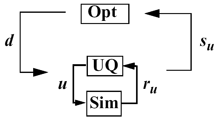
Fig. 57 Formulation 1: Nested OUU.
Listing 64 shows a Dakota input file for a nested OUU example problem that is based on the textbook test problem. In this example, the objective function contains two probability of failure estimates, and an inequality constraint contains another probability of failure estimate. For this example, failure is defined to occur when one of the textbook response functions exceeds its threshold value. The environment keyword block at the top of the input file identifies this as an OUU problem. The environment keyword block is followed by the optimization specification, consisting of the optimization method, the continuous design variables, and the response quantities that will be used by the optimizer. The mapping matrices used for incorporating UQ statistics into the optimization response data are described here.
The uncertainty quantification specification includes the UQ method, the uncertain variable probability distributions, the interface to the simulation code, and the UQ response attributes. As with other complex Dakota input files, the identification tags given in each keyword block can be used to follow the relationships among the different keyword blocks.
dakota/share/dakota/examples/users/textbook_opt_ouu1.in# Dakota Input File: textbook_opt_ouu1.in
environment
top_method_pointer = 'OPTIM'
method
id_method = 'OPTIM'
## (NPSOL requires a software license; if not available, try
## conmin_mfd or optpp_q_newton instead)
npsol_sqp
convergence_tolerance = 1.e-10
model_pointer = 'OPTIM_M'
model
id_model = 'OPTIM_M'
nested
sub_method_pointer = 'UQ'
primary_response_mapping = 0. 0. 1. 0. 0. 1. 0. 0. 0.
secondary_response_mapping = 0. 0. 0. 0. 0. 0. 0. 0. 1.
variables_pointer = 'OPTIM_V'
responses_pointer = 'OPTIM_R'
variables
id_variables = 'OPTIM_V'
continuous_design = 2
initial_point 1.8 1.0
upper_bounds 2.164 4.0
lower_bounds 1.5 0.0
descriptors 'd1' 'd2'
responses
id_responses = 'OPTIM_R'
objective_functions = 1
nonlinear_inequality_constraints = 1
upper_bounds = .1
numerical_gradients
method_source dakota
interval_type central
fd_step_size = 1.e-1
no_hessians
method
id_method = 'UQ'
sampling
model_pointer = 'UQ_M'
samples = 50 sample_type lhs
seed = 1
response_levels = 3.6e+11 1.2e+05 3.5e+05
distribution complementary
model
id_model = 'UQ_M'
single
interface_pointer = 'UQ_I'
variables_pointer = 'UQ_V'
responses_pointer = 'UQ_R'
variables
id_variables = 'UQ_V'
continuous_design = 2
normal_uncertain = 2
means = 248.89 593.33
std_deviations = 12.4 29.7
descriptors = 'nuv1' 'nuv2'
uniform_uncertain = 2
lower_bounds = 199.3 474.63
upper_bounds = 298.5 712.
descriptors = 'uuv1' 'uuv2'
weibull_uncertain = 2
alphas = 12. 30.
betas = 250. 590.
descriptors = 'wuv1' 'wuv2'
interface
id_interface = 'UQ_I'
analysis_drivers = 'text_book_ouu'
direct
# fork asynch evaluation_concurrency = 5
responses
id_responses = 'UQ_R'
response_functions = 3
no_gradients
no_hessians
Latin hypercube sampling is used as the UQ method in this example problem. Thus, each evaluation of the response functions by the optimizer entails 50 Latin hypercube samples. In general, nested OUU studies can easily generate several thousand function evaluations and gradient-based optimizers may not perform well due to noisy or insensitive statistics resulting from under-resolved sampling. These observations motivate the use of surrogate-based approaches to OUU.
Other nested OUU examples in the directory
dakota/share/dakota/test include dakota_ouu1_tbch.in, which
adds an additional interface for including deterministic data in the
textbook OUU problem, and dakota_ouu1_cantilever.in, which solves
the cantilever OUU problem with a
nested approach. For each of these files, the “1” identifies
formulation 1, which is short-hand for the nested approach.
Surrogate-Based OUU (SBOUU)
Surrogate-based optimization under uncertainty strategies can be effective in reducing the expense of OUU studies. Possible formulations include use of a surrogate model at the optimization level, at the uncertainty quantification level, or at both levels. These surrogate models encompass both data fit surrogates (at the optimization or UQ level) and model hierarchy surrogates (at the UQ level only). Fig. 58 depicts the different surrogate-based formulations where \(\mathbf{\hat{r}_{u}}\) and \(\mathbf{\hat{s}_{u}}\) are approximate response functions and approximate response statistics, respectively, generated from the surrogate models.
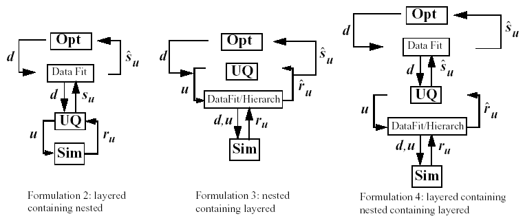
Fig. 58 Formulations 2, 3, and 4 for Surrogate-based OUU.
SBOUU examples in the dakota/share/dakota/test directory include
dakota_sbouu2_tbch.in, dakota_sbouu3_tbch.in, and
dakota_sbouu4_tbch.in, which solve the textbook OUU problem, and
dakota_sbouu2_cantilever.in, dakota_sbouu3_cantilever.in, and
dakota_sbouu4_cantilever.in, which solve the cantilever OUU problem.
For each of these files, the “2,” “3,” and “4” identify formulations
2, 3, and 4, which are short-hand for the “layered containing nested,”
“nested containing layered,” and “layered containing nested containing
layered” surrogate-based formulations, respectively. In general, the use
of surrogates greatly reduces the computational expense of these OUU
study. However, without restricting and verifying the steps in the
approximate optimization cycles, weaknesses in the data fits can be
exploited and poor solutions may be obtained. The need to maintain
accuracy of results leads to the use of trust-region surrogate-based
approaches.
Trust-Region Surrogate-Based OUU (TR-SBOUU)
The TR-SBOUU approach applies the trust region logic of deterministic SBO to SBOUU. Trust-region verifications are applicable when surrogates are used at the optimization level, i.e., formulations 2 and 4. As a result of periodic verifications and surrogate rebuilds, these techniques are more expensive than SBOUU; however they are more reliable in that they maintain the accuracy of results. Relative to nested OUU (formulation 1), TR-SBOUU tends to be less expensive and less sensitive to initial seed and starting point.
TR-SBOUU examples in the directory dakota/share/dakota/test
include dakota_trsbouu2_tbch.in and dakota_trsbouu4_tbch.in,
which solve the textbook OUU problem, and
dakota_trsbouu2_cantilever.in and
dakota_trsbouu4_cantilever.in, which solve the cantilever OUU problem.
Computational results for several example problems are available in [EGWojtkiewiczJrT02].
RBDO
Bi-level and sequential approaches to reliability-based design optimization (RBDO) and their associated sensitivity analysis requirements are described in the Optimization Under Uncertainty theory section.
A number of bi-level RBDO examples are provided in
dakota/share/dakota/test. The dakota_rbdo_cantilever.in,
dakota_rbdo_short_column.in, and dakota_rbdo_steel_column.in
input files solve the cantilever,
short column, and
steel column OUU
problems using a bi-level RBDO approach employing numerical design
gradients. The dakota_rbdo_cantilever_analytic.in and
dakota_rbdo_short_column_analytic.in input files solve the
cantilever and short column OUU problems using a bi-level RBDO
approach with analytic design gradients and first-order limit state
approximations. The dakota_rbdo_cantilever_analytic2.in,
dakota_rbdo_short_column_analytic2.in, and
dakota_rbdo_steel_column_analytic2.in input files also employ
analytic design gradients, but are extended to employ second-order
limit state approximations and integrations.
Sequential RBDO examples are also provided in
dakota/share/dakota/test. The dakota_rbdo_cantilever_trsb.in
and dakota_rbdo_short_column_trsb.in input files solve the
cantilever and short column OUU problems using a first-order
sequential RBDO approach with analytic design gradients and
first-order limit state approximations. The
dakota_rbdo_cantilever_trsb2.in,
dakota_rbdo_short_column_trsb2.in, and
dakota_rbdo_steel_column_trsb2.in input files utilize second-order
sequential RBDO approaches that employ second-order limit state
approximations and integrations (from analytic limit state Hessians with
respect to the uncertain variables) and quasi-Newton approximations to
the reliability metric Hessians with respect to design variables.
Stochastic Expansion-Based Design Optimization
For stochastic expansion-based approaches to optimization under uncertainty, bi-level, sequential, and multifidelity approaches and their associated sensitivity analysis requirements are described in the Optimization Under Uncertainty theory section.
In dakota/share/dakota/test, the dakota_pcbdo_cantilever.in,
dakota_pcbdo_rosenbrock.in, dakota_pcbdo_short_column.in, and
dakota_pcbdo_steel_column.in input files solve cantilever,
Rosenbrock, short column, and
steel column OUU
problems using a bi-level polynomial chaos-based approach, where the
statistical design metrics are reliability indices based on moment
projection (see the Mean Value section in Reliability Methods theory section). The test matrix in
the former three input files evaluate design gradients of these
reliability indices using several different approaches: analytic design
gradients based on a PCE formed over only over the random variables,
analytic design gradients based on a PCE formed over all variables,
numerical design gradients based on a PCE formed only over the random
variables, and numerical design gradients based on a PCE formed over all
variables. In the cases where the expansion is formed over all
variables, only a single PCE construction is required for the complete
PCBDO process, whereas the expansions only over the random variables
must be recomputed for each change in design variables. Sensitivities
for “augmented” design variables (which are separate from and augment
the random variables) may be handled using either analytic approach;
however, sensitivities for “inserted” design variables (which define
distribution parameters for the random variables) must be
computed using \(\frac{dR}{dx} \frac{dx}{ds}\) (refer to Stochastic Sensitivity Analysis section in the Optimization Under Uncertainty theory section).
Additional test input files include:
dakota_scbdo_cantilever.in,dakota_scbdo_rosenbrock.in,dakota_scbdo_short_column.in, anddakota_scbdo_steel_column.ininput files solve cantilever, Rosenbrock, short column, and steel column OUU problems using a bi-level stochastic collocation-based approach.dakota_pcbdo_cantilever_trsb.in,dakota_pcbdo_rosenbrock_trsb.in,dakota_pcbdo_short_column_trsb.in,dakota_pcbdo_steel_column_trsb.in,dakota_scbdo_cantilever_trsb.in,dakota_scbdo_rosenbrock_trsb.in,dakota_scbdo_short_column_trsb.in, anddakota_scbdo_steel_column_trsb.ininput files solve cantilever, Rosenbrock, short column, and steel column OUU problems using sequential polynomial chaos-based and stochastic collocation-based approaches.dakota_pcbdo_cantilever_mf.in,dakota_pcbdo_rosenbrock_mf.in,dakota_pcbdo_short_column_mf.in,dakota_scbdo_cantilever_mf.in,dakota_scbdo_rosenbrock_mf.in, anddakota_scbdo_short_column_mf.ininput files solve cantilever, Rosenbrock, and short column OUU problems using multifidelity polynomial chaos-based and stochastic collocation-based approaches.
Epistemic OUU
An emerging capability is optimization under epistemic uncertainty. As described in the section on nested models, epistemic and mixed aleatory/epistemic uncertainty quantification methods generate lower and upper interval bounds for all requested response, probability, reliability, and generalized reliability level mappings. Design for robustness in the presence of epistemic uncertainty could simply involve minimizing the range of these intervals (subtracting lower from upper using the nested model response mappings), and design for reliability in the presence of epistemic uncertainty could involve controlling the worst case upper or lower bound of the interval.
We now have the capability to perform epistemic analysis by using
interval optimization on the “outer loop” to calculate bounding
statistics of the aleatory uncertainty on the “inner loop.” Preliminary
studies [ES09] have shown this approach is more
efficient and accurate than nested sampling, which was described in
the example from this section. This approach uses an
efficient global optimization method for the outer loop and stochastic
expansion methods (e.g. polynomial chaos or stochastic collocation on
the inner loop). The interval optimization is described here.
Example input files demonstrating the use of interval estimation for epistemic analysis,
specifically in epistemic-aleatory nesting, are:
dakota_uq_cantilever_sop_exp.in, and dakota_short_column_sop_exp.in.
Both files are in dakota/share/dakota/test.
Surrogate-Based Uncertainty Quantification
Many uncertainty quantification (UQ) methods are computationally costly. For example, sampling often requires many function evaluations to obtain accurate estimates of moments or percentile values of an output distribution. One approach to overcome the computational cost of sampling is to evaluate the true function (e.g. run the analysis driver) on a fixed, small set of samples, use these sample evaluations to create a response surface approximation (e.g. a surrogate model or meta-model) of the underlying “true” function, then perform random sampling (using thousands or millions of samples) on the approximation to obtain estimates of the mean, variance, and percentiles of the response.
This approach, called “surrogate-based uncertainty quantification” is
easy to do in Dakota, and one can set up input files to compare the
results using no approximation (e.g. determine the mean, variance, and
percentiles of the output directly based on the initial sample values)
with the results obtained by sampling a variety of surrogate
approximations. Example input files of a standard UQ analysis based on
sampling alone vs. sampling a surrogate are shown in
textbook_uq_sampling.in and textbook_uq_surrogate.in in the
dakota/share/dakota/examples/users directory.
Note that one must exercise some caution when using surrogate-based methods for uncertainty quantification. In general, there is not a single, straightforward approach to incorporate the error of the surrogate fit into the uncertainty estimates of the output produced by sampling the surrogate. Two references which discuss some of the related issues are [GMSE06] and [SSG06]. The first reference shows that statistics of a response based on a surrogate model were less accurate, and sometimes biased, for surrogates constructed on very small sample sizes. In many cases, however, [GMSE06] shows that surrogate-based UQ performs well and sometimes generates more accurate estimates of statistical quantities on the output. The second reference goes into more detail about the interaction between sample type and response surface type (e.g., are some response surfaces more accurate when constructed on a particular sample type such as LHS vs. an orthogonal array?) In general, there is not a strong dependence of the surrogate performance with respect to sample type, but some sample types perform better with respect to some metrics and not others (for example, a Hammersley sample may do well at lowering root mean square error of the surrogate fit but perform poorly at lowering the maximum absolute deviation of the error). Much of this work is empirical and application dependent. If you choose to use surrogates in uncertainty quantification, we strongly recommend trying a variety of surrogates and examining diagnostic goodness-of-fit metrics.
Warning
Known Issue: When using discrete variables, there have been sometimes significant differences in data fit surrogate behavior observed across computing platforms in some cases. The cause has not yet been fully diagnosed and is currently under investigation. In addition, guidance on appropriate construction and use of surrogates with discrete variables is under development. In the meantime, users should therefore be aware that there is a risk of inaccurate results when using surrogates with discrete variables.