Parallel Computing
Overview
This chapter describes the various parallel computing capabilities provided by Dakota. We begin with a high-level summary.
Dakota has been designed to exploit a wide range of parallel computing resources such as those found in a desktop multiprocessor workstation, a network of workstations, or a massively parallel computing platform. This parallel computing capability is a critical technology for rendering real-world engineering design problems computationally tractable. Dakota employs the concept of multilevel parallelism, which takes simultaneous advantage of opportunities for parallel execution from multiple sources:
Parallel Simulation Codes: Dakota works equally well with both serial and parallel simulation codes.
Concurrent Execution of Analyses within a Function Evaluation: Some engineering design applications call for the use of multiple simulation code executions (different disciplinary codes, the same code for different load cases or environments, etc.) in order to evaluate a single response data set (e.g., objective functions and constraints) for a single set of parameters. If these simulation code executions are independent (or if coupling is enforced at a higher level), Dakota can perform them concurrently.
Concurrent Execution of Function Evaluations within an Iterator: Many Dakota methods provide opportunities for the concurrent evaluation of response data sets for different parameter sets. Whenever there exists a set of function evaluations that are independent, Dakota can perform them in parallel.
Note
The term function evaluation is used broadly to mean any individual data request from an iterative algorithm
Concurrent Execution of Sub-Iterators within a Meta-iterator or Nested Model: The advanced methods described on the Advanced Methods page are examples of meta-iterators, and the advanced model recursions described on the Advanced Models page all utilize nested models. Both of these cases generate sets of iterator subproblems that can be executed concurrently. For example, the Pareto-set and multi-start strategies generate sets of optimization subproblems. Similarly, optimization under uncertainty generates sets of uncertainty quantification subproblems. Whenever these subproblems are independent, Dakota can perform them in parallel.
It is important to recognize that these four parallelism sources can be combined recursively. For example, a meta-iterator can schedule and manage concurrent iterators, each of which may manage concurrent function evaluations, each of which may manage concurrent analyses, each of which may execute on multiple processors. Moreover, more than one source of sub-iteration concurrency can be exploited when combining meta-iteration and nested model sources. In an extreme example, defining the Pareto frontier for mixed-integer nonlinear programming under mixed aleatory-epistemic uncertainty might exploit up to four levels of nested sub-iterator concurrency in addition to available levels from function evaluation concurrency, analysis concurrency, and simulation parallelism. The majority of application scenarios, however, will employ one to two levels of parallelism.
Navigating the body of this chapter: The range of capabilities is extensive and can be daunting at first; therefore, this chapter takes an incremental approach in first describing the simplest single-level parallel computing models using asynchronous local, message passing, and hybrid approaches. More advanced uses of Dakota can build on this foundation to exploit multiple levels of parallelism.
The chapter concludes with a discussion of using Dakota with applications that run as independent MPI processes (parallel application tiling, for example on a large compute cluster). This last section is a good quick start for interfacing Dakota to your parallel (or serial) application on a cluster.
Categorization of parallelism
To understand the parallel computing possibilities, it is instructive to first categorize the opportunities for exploiting parallelism into four main areas [EH98], consisting of coarse-grained and fine-grained parallelism opportunities within algorithms and their function evaluations:
Algorithmic coarse-grained parallelism: This parallelism involves the concurrent execution of independent function evaluations, where a “function evaluation” is defined as a data request from an algorithm (which may involve value, gradient, and Hessian data from multiple objective and constraint functions). This concept can also be extended to the concurrent execution of multiple “iterators” within a “meta-iterator.” Examples of algorithms containing coarse-grained parallelism include:
Gradient-based algorithms: finite difference gradient evaluations, speculative optimization, parallel line search.
Nongradient-based algorithms: genetic algorithms (GAs), pattern search (PS), Monte Carlo sampling.
Approximate methods: design of computer experiments for building surrogate models.
Concurrent sub-iteration: optimization under uncertainty, branch and bound, multi-start local search, Pareto set optimization, island-model GAs.
Algorithmic fine-grained parallelism: This involves computing the basic computational steps of an optimization algorithm (i.e., the internal linear algebra) in parallel. This is primarily of interest in large-scale optimization problems and simultaneous analysis and design (SAND).
Function evaluation coarse-grained parallelism: This involves concurrent computation of separable parts of a single function evaluation. This parallelism can be exploited when the evaluation of the response data set requires multiple independent simulations (e.g. multiple loading cases or operational environments) or multiple dependent analyses where the coupling is applied at the optimizer level (e.g., multiple disciplines in the individual discipline feasible formulation [DL94]).
Function evaluation fine-grained parallelism: This involves parallelization of the solution steps within a single analysis code. Support for massively parallel simulation continues to grow in areas of nonlinear mechanics, structural dynamics, heat transfer, computational fluid dynamics, shock physics, and many others.
By definition, coarse-grained parallelism requires very little inter-processor communication and is therefore “embarrassingly parallel,” meaning that there is little loss in parallel efficiency due to communication as the number of processors increases. However, it is often the case that there are not enough separable computations on each algorithm cycle to utilize the thousands of processors available on massively parallel machines. For example, a thermal safety application [EHB+96] demonstrated this limitation with a pattern search optimization in which the maximum speedup exploiting only coarse-grained algorithmic parallelism was shown to be limited by the size of the design problem (coordinate pattern search has at most \(2n\) independent evaluations per cycle for \(n\) design variables).
Fine-grained parallelism, on the other hand, involves much more communication among processors and care must be taken to avoid the case of inefficient machine utilization in which the communication demands among processors outstrip the amount of actual computational work to be performed. For example, a chemically-reacting flow application [EH98] illustrated this limitation for a simulation of fixed size in which it was shown that, while simulation run time did monotonically decrease with increasing number of processors, the relative parallel efficiency \(\hat{E}\) of the computation for fixed model size decreased rapidly (from \(\hat{E} \approx 0.8\) at 64 processors to \(\hat{E} \approx 0.4\) at 512 processors). This was due to the fact that the total amount of computation was approximately fixed, whereas the communication demands were increasing rapidly with increasing numbers of processors. Therefore, there is a practical limit on the number of processors that can be employed for fine-grained parallel simulation of a particular model size, and only for extreme model sizes can thousands of processors be efficiently utilized in studies exploiting fine-grained parallelism alone.
These limitations point us to the exploitation of multiple levels of parallelism, in particular the combination of coarse-grained and fine-grained approaches. This will allow us to execute fine-grained parallel simulations on sets of processors where they are most efficient and then replicate this efficiency with many coarse-grained instances involving one or more levels of nested job scheduling.
Parallel Dakota algorithms
In Dakota, the following parallel algorithms, comprised of iterators and meta-iterators, provide support for coarse-grained algorithmic parallelism. Note that, even if a particular algorithm is serial in terms of its data request concurrency, other concurrency sources (e.g., function evaluation coarse-grained and fine-grained parallelism) may still be available.
Parallel iterators
Gradient-based optimizers: CONMIN, DOT, NLPQL, NPSOL, and OPT++ can all exploit parallelism through the use of Dakota’s native finite differencing routine (selected with in the responses specification), which will perform concurrent evaluations for each of the parameter offsets. For \(n\) variables, forward differences result in an \(n+1\) concurrency and central differences result in a \(2n+1\) concurrency. In addition, CONMIN, DOT, and OPT++ can use speculative gradient techniques [BSS88] to obtain better parallel load balancing. By speculating that the gradient information associated with a given line search point will be used later and computing the gradient information in parallel at the same time as the function values, the concurrency during the gradient evaluation and line search phases can be balanced. NPSOL does not use speculative gradients since this approach is superseded by NPSOL’s gradient-based line search in user-supplied derivative mode. NLPQL also supports a distributed line search capability for generating concurrency [Sch04]. Finally, finite-difference Newton algorithms can exploit additional concurrency in numerically evaluating Hessian matrices.
Nongradient-based optimizers: HOPSPACK, JEGA methods, and most SCOLIB methods support parallelism. HOPSPACK and SCOLIB methods exploit parallelism through the use of Dakota’s concurrent function evaluations; however, there are some limitations on the levels of concurrency and asynchrony that can be exploited. These are detailed in the Dakota Reference Manual. Serial SCOLIB methods include Solis-Wets (
coliny_solis_wets) and certainexploratory_movesoptions (adaptive_patternandmulti_step) in pattern search (coliny_pattern_search). OPT++ PDS and NCSU DIRECT are also currently serial due to incompatibilities in Dakota and OPT++/NCSU parallelism models. Finally, and support dynamic job queues managed with nonblocking synchronization.Least squares methods: in an identical manner to the gradient-based optimizers, NL2SOL, NLSSOL, and Gauss-Newton can exploit parallelism through the use of Dakota’s native finite differencing routine. In addition, NL2SOL and Gauss-Newton can use speculative gradient techniques to obtain better parallel load balancing. NLSSOL does not use speculative gradients since this approach is superseded by NLSSOL’s gradient-based line search in user-supplied derivative mode.
Surrogate-based minimizers:
surrogate_based_local,surrogate_based_global, andefficient_globalall support parallelism in the initial surrogate construction, but subsequent concurrency varies. In the case ofefficient_global, available concurrency depends onbatch_size. In the case ofsurrogate_based_local, only a single point is generated per subsequent cycle, but derivative concurrency for numerical gradient or Hessian evaluations may be available. And in the case ofsurrogate_based_global, multiple points may be generated on each subsequent cycle, depending on the multipoint return capability of specific minimizers.Parameter studies: all parameter study methods (vector, list, centered, and multidim) support parallelism. These methods avoid internal synchronization points, so all evaluations are available for concurrent execution.
Design of experiments: all
dace(grid,random,oas,lhs,oa_lhs,box_behnken, andcentral_composite),fsu_quasi_mc(haltonandhammersley),fsu_cvt, andpsuade_moatmethods support parallelism.Uncertainty quantification: all nondeterministic methods (
sampling, reliability, stochastic expansion, and epistemic) support parallelism. In the case of gradient-based methods (local_reliability,local_interval_est) parallelism can be exploited through the use of Dakota’s native finite differencing routine for computing gradients. In the case of many global methods (e.g.,global_reliability,global_interval_est,polynomial_chaos) initial surrogate construction is highly parallel, but any subsequent (adaptive) refinement may have greater concurrency restrictions (including a single point per refinement cycle in some cases).
Advanced methods
Certain advanced methods support concurrency in multiple iterator executions. Currently, the methods which can exploit this level of parallelism are:
Hybrid minimization: when the sequential hybrid transfers multiple solution points between methods, single-point minimizers will be executed concurrently using each of the transferred solution points.
Pareto-set optimization: a meta-iterator for multiobjective optimization using the simple weighted-sum approach for computing sets of points on the Pareto front of nondominated solutions.
Multi-start iteration: a meta-iterator for executing multiple instances of an iterator from different starting points.
The hybrid minimization case will display varying levels of iterator concurrency based on differing support of multipoint solution input/output between iterators; however, the use of multiple parallel configurations among the iterator sequence should prevent parallel inefficiencies. On the other hand, pareto-set and multi-start have a fixed set of jobs to perform and should exhibit good load balancing.
Parallel models
Parallelism support in model is an important issue for advanced model recursions such as surrogate-based minimization, optimization under uncertainty, and mixed aleatory-epistemic UQ (see the Advanced Method and Advanced Model pages). Support is as follows:
Single model: parallelism is managed as specified in the model’s associated
interfaceinstance.Recast model: most parallelism is forwarded on to the sub-model. An exception to this is finite differencing in the presence of variable scaling. Since it is desirable to perform offsets in the scaled space (and avoid minimum step size tolerances), this parallelism is not forwarded to the sub-model, instead being enacted at the recast level.
Data fit surrogate model: parallelism is supported in the construction of global surrogate models via the concurrent evaluation of points generated by design of experiments methods. Local and multipoint approximations evaluate only a single point at a time, so concurrency is available only from any numerical differencing required for gradient and Hessian data. Since the top-level iterator is interfaced only with the (inexpensive) surrogate, no parallelism is exploited there. Load balancing can be an important issue when performing evaluations to (adaptively) update existing surrogate models.
Hierarchical surrogate model: parallelism is supported for the low or the high fidelity models, and in some contexts, for both models at the same time. In the multifidelity optimization context, the optimizer is interfaced only with the low-fidelity model, and the high-fidelity model is used only for verifications and correction updating. For this case, the algorithmic coarse-grained parallelism supported by the optimizer is enacted on the low fidelity model and the only parallelism available for high fidelity executions arises from any numerical differencing required for high-fidelity gradient and Hessian data. In contexts that compute model discrepancies, such as multifidelity UQ, the algorithmic concurrency involves evaluation of both low and high fidelity models, so parallel schedulers can exploit simultaneous concurrency for both models.
Nested model: concurrent executions of the optional interface and concurrent executions of the sub-iterator are supported and are synchronized in succession. Currently, synchronization is blocking (all concurrent evaluations are completed before new batches are scheduled); nonblocking schedulers (see Single-level parallelism) may be supported in time. Nested model concurrency and meta-iterator concurrency (Advanced methods) may be combined within an arbitrary number of levels of recursion. Primary clients for this capability include optimization under uncertainty and mixed aleatory-epistemic UQ.
Single-level parallelism
Dakota’s parallel facilities support a broad range of computing hardware, from custom massively parallel supercomputers on the high end, to clusters and networks of workstations in the middle range, to desktop multiprocessors on the low end. Given the reduced scale in the middle to low ranges, it is more common to exploit only one of the levels of parallelism; however, this can still be quite effective in reducing the time to obtain a solution. Three single-level parallelism models will be discussed, and are depicted in Fig. 59:
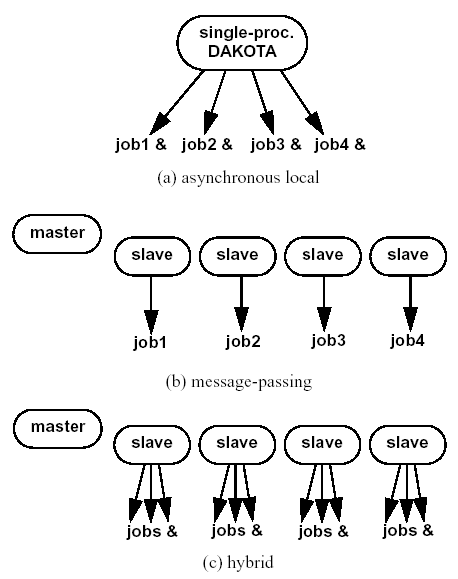
Fig. 59 External, internal, and hybrid job management.
asynchronous local: Dakota executes on a single processor, but launches multiple jobs concurrently using asynchronous job launching techniques.
message passing: Dakota executes in parallel using message passing to communicate between processors. A single job is launched per processor using synchronous job launching techniques.
hybrid: a combination of message passing and asynchronous local. Dakota executes in parallel across multiple processors and launches concurrent jobs on each processor.
In each of these cases, jobs are executing concurrently and must be collected in some manner for return to an algorithm. Blocking and nonblocking approaches are provided for this, where the blocking approach is used in most cases:
blocking synchronization: all jobs in the queue are completed before exiting the scheduler and returning the set of results to the algorithm. The job queue fills and then empties completely, which provides a synchronization point for the algorithm.
nonblocking synchronization: the job queue is dynamic, with jobs entering and leaving continuously. There are no defined synchronization points for the algorithm, which requires specialized algorithm logic. Sometimes referred to as “fully asynchronous” algorithms, these currently include
coliny_pattern_search,asynch_pattern_search, andefficient_globalwith thenonblockingoption.
Given these job management capabilities, it is worth noting that the popular term “asynchronous” can be ambiguous when used in isolation. In particular, it can be important to qualify whether one is referring to “asynchronous job launch” (synonymous with any of the three concurrent job launch approaches described above) or “asynchronous job recovery” (synonymous with the latter nonblocking job synchronization approach).
Asynchronous Local Parallelism
This section describes software components which manage simulation invocations local to a processor. These invocations may be either synchronous (i.e., blocking) or asynchronous (i.e., nonblocking). Synchronous evaluations proceed one at a time with the evaluation running to completion before control is returned to Dakota. Asynchronous evaluations are initiated such that control is returned to Dakota immediately, prior to evaluation completion, thereby allowing the initiation of additional evaluations which will execute concurrently.
The synchronous local invocation capabilities are used in two contexts: (1) by themselves to provide serial execution on a single processor, and (2) in combination with Dakota’s message-passing schedulers to provide function evaluations local to each processor. Similarly, the asynchronous local invocation capabilities are used in two contexts: (1) by themselves to launch concurrent jobs from a single processor that rely on external means (e.g., operating system, job queues) for assignment to other processors, and (2) in combination with Dakota’s message-passing schedulers to provide a hybrid parallelism. Thus, Dakota supports any of the four combinations of synchronous or asynchronous local combined with message passing or without.
Asynchronous local schedulers may be used for managing concurrent
function evaluations requested by an iterator or for managing concurrent
analyses within each function evaluation. The former iterator/evaluation
concurrency supports either blocking (all jobs in the queue must be
completed by the scheduler) or nonblocking (dynamic job queue may shrink
or expand) synchronization, where blocking synchronization is used by
most iterators and nonblocking synchronization is used by fully
asynchronous algorithms such as asynch_pattern_search,
coliny_pattern_search, and efficient_global
with the nonblocking option.
The latter evaluation/analysis concurrency is
restricted to blocking synchronization. The “Asynchronous Local” column
in Table 14 summarizes these capabilities.
Dakota supports three local simulation invocation approaches based on the direct function, system call, and fork simulation interfaces. For each of these cases, an input filter, one or more analysis drivers, and an output filter make up the interface, as described in Simulation Interface Components.
Direct function synchronization
The direct function capability may be used synchronously. Synchronous operation of the direct function simulation interface involves a standard procedure call to the input filter, if present, followed by calls to one or more simulations, followed by a call to the output filter, if present (refer to Simulation Interface Components for additional details and examples). Each of these components must be linked as functions within Dakota. Control does not return to the calling code until the evaluation is completed and the response object has been populated.
Asynchronous operation will be supported in the future and will involve
the use of multithreading (e.g., POSIX threads) to accomplish multiple
simultaneous simulations. When spawning a thread (e.g., using
pthread_create), control returns to the calling code after the
simulation is initiated. In this way, multiple threads can be created
simultaneously. An array of responses corresponding to the multiple
threads of execution would then be recovered in a synchronize operation
(e.g., using pthread_join).
System call synchronization
The system call capability may be used synchronously or asynchronously.
In both cases, the system utility from the standard C library is
used. Synchronous operation of the system call simulation interface
involves spawning the system call (containing the filters and analysis
drivers bound together with parentheses and semi-colons) in the
foreground. Control does not return to the calling code until the
simulation is completed and the response file has been written. In this
case, the possibility of a race condition (see below) does not exist and
any errors during response recovery will cause an immediate abort of the
Dakota process.
Note
Detection of the string “fail” is not a response recovery error; see Simulation Failure Capturing.
Asynchronous operation involves spawning the system call in the background, continuing with other tasks (e.g., spawning other system calls), periodically checking for process completion, and finally retrieving the results. An array of responses corresponding to the multiple system calls is recovered in a synchronize operation.
In this synchronize operation, completion of a function evaluation is
detected by testing for the existence of the evaluation’s results file
using the stat utility [KR88]. Care must be taken
when using asynchronous system calls since they are prone to the race
condition in which the results file passes the existence test but the
recording of the function evaluation results in the file is incomplete.
In this case, the read operation performed by Dakota will result in an
error due to an incomplete data set. In order to address this problem,
Dakota contains exception handling which allows for a fixed number of
response read failures per asynchronous system call evaluation. The
number of allowed failures must have a limit, so that an actual response
format error (unrelated to the race condition) will eventually abort the
system. Therefore, to reduce the possibility of exceeding the limit on
allowable read failures, the user’s interface should minimize the
amount of time an incomplete results file exists in the directory where
its status is being tested. This can be accomplished through two
approaches: (1) delay the creation of the results file until the
simulation computations are complete and all of the response data is
ready to be written to the results file, or (2) perform the simulation
computations in a subdirectory, and as a last step, move the completed
results file into the main working directory where its existence is
being queried.
If concurrent simulations are executing in a shared disk space, then
care must be taken to maintain independence of the simulations. In
particular, the parameters and results files used to communicate between
Dakota and the simulation, as well as any other files used by this
simulation, must be protected from other files of the same name used by
the other concurrent simulations. With respect to the parameters and
results files, these files may be made unique through the use of the
file_tag option (e.g., params.in.1, results.out.1)
or the default temporary file option (e.g.,
/var/tmp/aaa0b2Mfv). However, if additional simulation files must
be protected (e.g., model.i, model.o, model.g,
model.e), then an effective approach is to create
a tagged working subdirectory for each simulation instance.
The Interfaces page provides an
example system call interface that demonstrates both the use of tagged
working directories and the relocation of completed results files to
avoid the race condition.
Fork synchronization
The fork capability is quite similar to the system call; however, it has
the advantage that asynchronous fork invocations can avoid the results
file race condition that may occur with asynchronous system calls (See
the Interfaces page discussion on choosing
between fork and
system). The fork interface
invokes the filters and analysis drivers using the fork and exec
family of functions, and completion of these processes is detected using
the wait family of functions. Since wait is based on a process
id handle rather than a file existence test, an incomplete results file
is not an issue.
Depending on the platform, the fork simulation interface executes either
a vfork or a fork call. These calls generate a new child process
with its own UNIX process identification number, which functions as a
copy of the parent process (dakota). The execvp function is then
called by the child process, causing it to be replaced by the analysis
driver or filter. For synchronous operation, the parent dakota process
then awaits completion of the forked child process through a blocking
call to waitpid. On most platforms, the fork/exec procedure is
efficient since it operates in a copy-on-write mode, and no copy of the
parent is actually created. Instead, the parents address space is
borrowed until the exec function is called.
The fork/exec behavior for asynchronous operation is similar to that
for synchronous operation, the only difference being that dakota invokes
multiple simulations through the fork/exec procedure prior to
recovering response results for these jobs using the wait function.
The combined use of fork/exec and wait functions in asynchronous
mode allows the scheduling of a specified number of concurrent function
evaluations and/or concurrent analyses.
Asynchronous Local Example
The test file dakota/share/dakota/test/dakota_dace.in
computes 49 orthogonal array samples, which may be
evaluated concurrently using parallel computing. When executing Dakota
with this input file on a single processor, the following execution
syntax may be used:
dakota -i dakota_dace.in
For serial execution (the default), the interface specification within
dakota_dace.in would appear similar to
interface,
        system
          analysis_driver = 'text_book'
which results in function evaluation output similar to the following
(for output set to quiet mode):
>>>>> Running dace iterator.

DACE method = 12 Samples = 49 Symbols = 7 Seed (user-specified) = 5

------------------------------
Begin       I1 Evaluation    1
------------------------------
text_book /tmp/fileia6gVb /tmp/filedDo5MH

------------------------------
Begin       I1 Evaluation    2
------------------------------
text_book /tmp/fileyfkQGd /tmp/fileAbmBAJ

<snip>

<<<<< Iterator dace completed.
where it is evident that each function evaluation is being performed sequentially.
For parallel execution using asynchronous local approaches, the Dakota
execution syntax is unchanged as Dakota is still launched on a single
processor. However, the interface specification is augmented to
include the asynchronous keyword with optional concurrency limiter
to indicate that multiple analysis_driver instances will be
executed concurrently:
interface,
        system asynchronous evaluation_concurrency = 4
          analysis_driver = 'text_book'
which results in output excerpts similar to the following:
>>>>> Running dace iterator.

DACE method = 12 Samples = 49 Symbols = 7 Seed (user-specified) = 5

------------------------------
Begin       I1 Evaluation    1
------------------------------
(Asynchronous job 1 added to I1 queue)

------------------------------
Begin       I1 Evaluation    2
------------------------------
(Asynchronous job 2 added to I1 queue)

<snip>

------------------------------
Begin       I1 Evaluation   49
------------------------------
(Asynchronous job 49 added to I1 queue)

Blocking synchronize of 49 asynchronous evaluations
First pass: initiating 4 local asynchronous jobs
Initiating I1 evaluation 1
text_book /tmp/fileuLcfBp /tmp/file6XIhpm &
Initiating I1 evaluation 2
text_book /tmp/fileeC29dj /tmp/fileIdA22f &
Initiating I1 evaluation 3
text_book /tmp/fileuhCESc /tmp/fileajLgI9 &
Initiating I1 evaluation 4
text_book /tmp/filevJHMy6 /tmp/fileHFKip3 &
Second pass: scheduling 45 remaining local asynchronous jobs
Waiting on completed jobs
I1 evaluation 1 has completed
I1 evaluation 2 has completed
I1 evaluation 3 has completed
Initiating I1 evaluation 5
text_book /tmp/fileISsjh0 /tmp/fileSaek9W &
Initiating I1 evaluation 6
text_book /tmp/filefN271T /tmp/fileSNYVUQ &
Initiating I1 evaluation 7
text_book /tmp/filebAQaON /tmp/fileaMPpHK &
I1 evaluation 49 has completed

<snip>

<<<<< Iterator dace completed.
where it is evident that each of the 49 jobs is first queued and then a blocking synchronization is performed. This synchronization uses a simple scheduler that initiates 4 jobs and then replaces completing jobs with new ones until all 49 are complete.
The default job concurrency for asynchronous local parallelism is all
that is available from the algorithm (49 in this case), which could be
too many for the computational resources or their usage policies. The
concurrency level specification (4 in this case) instructs the scheduler
to keep 4 jobs running concurrently, which would be appropriate for,
e.g., a dual-processor dual-core workstation. In this case, it is the
operating system’s responsibility to assign the concurrent text_book
jobs to available processors/cores. Specifying greater concurrency than
that supported by the hardware will result in additional context
switching within a multitasking operating system and will generally
degrade performance. Note however that, in this example, there are a
total of 5 processes running, one for Dakota and four for the concurrent
function evaluations. Since the Dakota process checks periodically for
job completion and sleeps in between checks, it is relatively
lightweight and does not require a dedicated processor.
Local evaluation scheduling options
The default behavior for asynchronous local parallelism is for Dakota to
dispatch the next evaluation the local queue when one completes (and can
optionally be specified by
local_evaluation_scheduling dynamic.
In some cases, the simulation code interface benefits from knowing which
job number will replace a completed job. This includes some modes of
application tiling with certain MPI implementations, where sending a job
to the correct subset of available processors is done with relative node
scheduling. The keywords
local_evaluation_scheduling static
forces this behavior, so a completed evaluation will be replaced with one
congruent modulo the evaluation concurrency. For example, with 6
concurrent jobs, eval number 2 will be replaced with eval number 8.
Examples of this usage can be seen in
dakota/share/dakota/examples/parallelism.
Message Passing Parallelism
Dakota uses a “single program-multiple data” (SPMD) parallel programming model. It uses message-passing routines from the Message Passing Interface (MPI) standard [GLS94], [SOHL+96] to communicate data between processors. The SPMD designation simply denotes that the same Dakota executable is loaded on all processors during the parallel invocation. This differs from the MPMD model (“multiple program-multiple data”) which would have the Dakota executable on one or more processors communicating directly with simulator executables on other processors. The MPMD model has some advantages, but heterogeneous executable loads are not supported by all parallel environments. Moreover, the MPMD model requires simulation code intrusion on the same order as conversion to a subroutine, so subroutine conversion (see Developing a Direct Simulation Interface) in a direct-linked SPMD model is preferred.
Partitioning
A level of message passing parallelism can use either of two processor partitioning models:
Dedicated master: a single processor is dedicated to scheduling operations and the remaining processors are split into server partitions.
Peer partition: all processors are allocated to server partitions and the loss of a processor to scheduling is avoided.
These models are depicted in Fig. 60. The peer partition is desirable since it utilizes all processors for computation; however, it requires either the use of sophisticated mechanisms for distributed scheduling or a problem for which static scheduling of concurrent work performs well (see Scheduling below). If neither of these characteristics is present, then use of the dedicated master partition supports a dynamic scheduling which assures that server idleness is minimized.
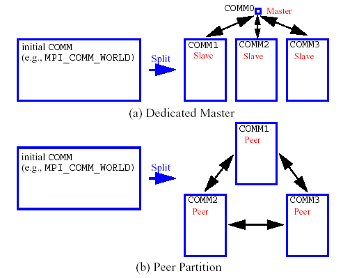
Fig. 60 Communicator partitioning models.
Scheduling
The following scheduling approaches are available within a level of message passing parallelism:
Dynamic scheduling: in the dedicated master model, the master processor manages a single processing queue and maintains a prescribed number of jobs (usually one) active on each slave. Once a slave server has completed a job and returned its results, the master assigns the next job to this slave. Thus, the job assignment on the master adapts to the job completion speed on the slaves. This provides a simple dynamic scheduler in that heterogeneous processor speeds and/or job durations are naturally handled, provided there are sufficient instances scheduled through the servers to balance the variation. In the case of a peer partition, dynamic schedulers can also be employed, provided that peer 1 can employ nonblocking synchronization of its local evaluations. This allows it to balance its local work with servicing job assignments and returns from the other peers.
Static scheduling: if scheduling is statically determined at start-up, then no master processor is needed to direct traffic and a peer partitioning approach is applicable. If the static schedule is a good one (ideal conditions), then this approach will have superior performance. However, heterogeneity, when not known a priori, can very quickly degrade performance since there is no mechanism to adapt.
Message passing schedulers may be used for managing concurrent
sub-iterator executions within a meta-iterator, concurrent evaluations
within an iterator, or concurrent analyses within an evaluation. In the
former and latter cases, the message passing scheduler is currently
restricted to blocking synchronization, in that all jobs in the queue
are completed before exiting the scheduler and returning the set of
results to the algorithm. Nonblocking message-passing scheduling is
supported for the iterator–evaluation concurrency level in support of
fully asynchronous algorithms (e.g., asynch_pattern_search,
coliny_pattern_search, and efficient_global)
that avoid synchronization points that can harm scaling.
Message passing is also used within a fine-grained parallel simulation code, although this is separate from Dakota’s capabilities (Dakota may, at most, pass a communicator partition to the simulation). The “Message Passing” column in Table 14 summarizes these capabilities.
Message Passing Example
Revisiting the test file dakota_dace.in,
Dakota will now compute the 49 orthogonal
array samples using a message passing approach. In this case, a parallel
launch utility is used to execute Dakota across multiple processors
using syntax similar to the following:
mpirun -np 5 -machinefile machines dakota -i dakota_dace.in
Since the asynchronous local parallelism will not be used, the
interface specification does not include the
asynchronous keyword and would appear similar to:
interface,
        system
          analysis_driver = 'text_book'
The relevant excerpts from the Dakota output for a dedicated master partition and dynamic schedule, the default when the maximum concurrency (49) exceeds the available capacity (5), would appear similar to the following:
Running MPI Dakota executable in parallel on 5 processors.
-----------------------------------------------------------------------------
DAKOTA parallel configuration:

Level                       num_servers    procs_per_server    partition
-----                       -----------    ----------------    ---------
concurrent evaluations           5                1            peer
concurrent analyses              1                1            peer
multiprocessor analysis          1               N/A           N/A

Total parallelism levels =   1 (1 dakota, 0 analysis)
-----------------------------------------------------------------------------
>>>>> Executing environment.

>>>>> Running dace iterator.

DACE method = 12 Samples = 49 Symbols = 7 Seed (user-specified) = 5

------------------------------
Begin       I1 Evaluation    1
------------------------------
(Asynchronous job 1 added to I1 queue)

------------------------------
Begin       I1 Evaluation    2
------------------------------
(Asynchronous job 2 added to I1 queue)

<snip>

------------------------------
Begin       I1 Evaluation   49
------------------------------
(Asynchronous job 49 added to I1 queue)

Blocking synchronize of 49 asynchronous evaluations
Peer dynamic schedule: first pass assigning 4 jobs among 4 remote peers
Peer 1 assigning I1 evaluation 1 to peer 2
Peer 1 assigning I1 evaluation 2 to peer 3
Peer 1 assigning I1 evaluation 3 to peer 4
Peer 1 assigning I1 evaluation 4 to peer 5
Peer dynamic schedule: first pass launching 1 local jobs
Initiating I1 evaluation 5
text_book /tmp/file5LRsBu /tmp/fileT2mS65 &
Peer dynamic schedule: second pass scheduling 44 remaining jobs
Initiating I1 evaluation 5
text_book /tmp/file5LRsBu /tmp/fileT2mS65 &
Peer dynamic schedule: second pass scheduling 44 remaining jobs
I1 evaluation 5 has completed
Initiating I1 evaluation 6
text_book /tmp/fileZJaODH /tmp/filewoUJaj &
I1 evaluation 2 has returned from peer server 3
Peer 1 assigning I1 evaluation 7 to peer 3
I1 evaluation 4 has returned from peer server 5

<snip>

I1 evaluation 46 has returned from peer server 2
I1 evaluation 49 has returned from peer server 5
<<<<< Function evaluation summary (I1): 49 total (49 new, 0 duplicate)

<<<<< Iterator dace completed.
where it is evident that each of the 49 jobs is first queued and then a blocking synchronization is performed. This synchronization uses a dynamic scheduler that initiates five jobs, one on each of five evaluation servers, and then replaces completing jobs with new ones until all 49 are complete. It is important to note that job execution local to each of the four servers is synchronous.
Hybrid Parallelism
The asynchronous local approaches described in the Asynchronous Local Parallelism section can be considered to rely on external scheduling mechanisms, since it is generally the operating system or some external queue/load sharing software that allocates jobs to processors. Conversely, the message-passing approaches described in Message Passing Parallelism rely on internal scheduling mechanisms to distribute work among processors. These two approaches provide building blocks which can be combined in a variety of ways to manage parallelism at multiple levels. At one extreme, Dakota can execute on a single processor and rely completely on external means to map all jobs to processors (i.e., using asynchronous local approaches). At the other extreme, Dakota can execute on many processors and manage all levels of parallelism, including the parallel simulations, using completely internal approaches (i.e., using message passing at all levels as in Fig. 63). While all-internal or all-external approaches are common cases, many additional approaches exist between the two extremes in which some parallelism is managed internally and some is managed externally.
These combined approaches are referred to as hybrid parallelism, since the internal distribution of work based on message-passing is being combined with external allocation using asynchronous local approaches.
Note
The term “hybrid parallelism” is often used to describe the combination of MPI message passing and OpenMP shared memory parallelism models. This can be considered to be a special case of the meaning here, as OpenMP is based on threads, which is analagous to asynchronous local usage of the direct simulation interface.
Fig. 59 depicts the asynchronous local, message-passing, and hybrid approaches for a dedicated-master partition. Approaches (b) and (c) both use MPI message-passing to distribute work from the master to the slaves, and approaches (a) and (c) both manage asynchronous jobs local to a processor. The hybrid approach (c) can be seen to be a combination of (a) and (b) since jobs are being internally distributed to slave servers through message-passing and each slave server is managing multiple concurrent jobs using an asynchronous local approach. From a different perspective, one could consider (a) and (b) to be special cases within the range of configurations supported by (c). The hybrid approach is useful for supercomputers that maintain a service/compute node distinction and for supercomputers or networks of workstations that involve clusters of symmetric multiprocessors (SMPs). In the service/compute node case, concurrent multiprocessor simulations are launched into the compute nodes from the service node partition. While an asynchronous local approach from a single service node would be sufficient, spreading the application load by running Dakota in parallel across multiple service nodes results in better performance [EHSvanBWaanders00]. If the number of concurrent jobs to be managed in the compute partition exceeds the number of available service nodes, then hybrid parallelism is the preferred approach. In the case of a cluster of SMPs (or network of multiprocessor workstations), message-passing can be used to communicate between SMPs, and asynchronous local approaches can be used within an SMP. Hybrid parallelism can again result in improved performance, since the total number of Dakota MPI processes is reduced in comparison to a pure message-passing approach over all processors.
Hybrid schedulers may be used for managing concurrent evaluations within an iterator or concurrent analyses within an evaluation. In the former case, blocking or nonblocking synchronization can be used, whereas the latter case is restricted to blocking synchronization. The “Hybrid” column in Table 14 summarizes these capabilities.
Hybrid Example
Revisiting the test file dakota_dace.in,
Dakota will now compute the 49 orthogonal
array samples using a hybrid approach. As for the message passing case,
a parallel launch utility is used to execute Dakota across multiple
processors:
mpirun -np 5 -machinefile machines dakota -i dakota_dace.in
Since the asynchronous local parallelism will also be used, the
interface specification includes the asynchronous
keyword and appears similar to
interface,
        system asynchronous evaluation_concurrency = 2
          analysis_driver = 'text_book'
In the hybrid case, the specification of the desired concurrency level must be included, since the default is no longer all available (as it is for asynchronous local parallelism). Rather the default is to employ message passing parallelism, and hybrid parallelism is only available through the specification of asynchronous concurrency greater than one.
The relevant excerpts of the Dakota output for a peer partition and dynamic schedule , the default when the maximum concurrency (49) exceeds the maximum available capacity (10), would appear similar to the following:
Running MPI Dakota executable in parallel on 5 processors.

-----------------------------------------------------------------------------
DAKOTA parallel configuration:

Level           num_servers    procs_per_server    partition
-----           -----------    ----------------    ---------
concurrent evaluations           5                1            peer
concurrent analyses              1                1            peer
multiprocessor analysis          1               N/A           N/A

Total parallelism levels =   1 (1 dakota, 0 analysis)
-----------------------------------------------------------------------------

>>>>> Executing environment.

>>>>> Running dace iterator.

DACE method = 12 Samples = 49 Symbols = 7 Seed (user-specified) = 5

------------------------------
Begin       I1 Evaluation    1
------------------------------
(Asynchronous job 1 added to I1 queue)

------------------------------
Begin       I1 Evaluation    2
------------------------------
(Asynchronous job 2 added to I1 queue)

<snip>

Blocking synchronize of 49 asynchronous evaluations
Peer dynamic schedule: first pass assigning 8 jobs among 4 remote peers
Peer 1 assigning I1 evaluation 1 to peer 2
Peer 1 assigning I1 evaluation 2 to peer 3
Peer 1 assigning I1 evaluation 3 to peer 4
Peer 1 assigning I1 evaluation 4 to peer 5
Peer 1 assigning I1 evaluation 6 to peer 2
Peer 1 assigning I1 evaluation 7 to peer 3
Peer 1 assigning I1 evaluation 8 to peer 4
Peer 1 assigning I1 evaluation 9 to peer 5
Peer dynamic schedule: first pass launching 2 local jobs
Initiating I1 evaluation 5
text_book /tmp/fileJU1Ez2 /tmp/fileVGZzEX &
Initiating I1 evaluation 10
text_book /tmp/fileKfUgKS /tmp/fileMgZXPN &
Peer dynamic schedule: second pass scheduling 39 remaining jobs

<snip>

I1 evaluation 49 has completed
I1 evaluation 43 has returned from peer server 2
I1 evaluation 44 has returned from peer server 3
I1 evaluation 48 has returned from peer server 4
I1 evaluation 47 has returned from peer server 2
I1 evaluation 45 has returned from peer server 3
<<<<< Function evaluation summary (I1): 49 total (49 new, 0 duplicate)

<<<<< Iterator dace completed.
where it is evident that each of the 49 jobs is first queued and then a blocking synchronization is performed. This synchronization uses a dynamic scheduler that initiates ten jobs, two on each of five evaluation servers, and then replaces completing jobs with new ones until all 49 are complete. It is important to note that job execution local to each of the four servers is asynchronous.
Multilevel parallelism
Parallel computing resources within the Department of Energy national laboratories continue to rapidly grow. In order to harness the power of these machines for performing design, uncertainty quantification, and other systems analyses, parallel algorithms are needed which are scalable to thousands of processors.
Dakota supports an open-ended number of levels of nested parallelism which, as described in the Overview above, can be categorized into three types of concurrent job scheduling and four types of parallelism: (a) concurrent iterators within a meta-iterator (scheduled by Dakota), (b) concurrent function evaluations within each iterator (scheduled by Dakota), (c) concurrent analyses within each function evaluation (scheduled by Dakota), and (d) multiprocessor analyses (work distributed by a parallel analysis code). In combination, these parallelism levels can minimize efficiency losses and achieve near linear scaling on MP computers. Types (a) and (b) are classified as algorithmic coarse-grained parallelism, type (c) is function evaluation coarse-grained parallelism, and type (d) is function evaluation fine-grained parallelism (see Categorization of parallelism). Algorithmic fine-grained parallelism is not currently supported in Dakota, although this picture is rapidly evolving.
A particular application may support one or more of these parallelism types, and Dakota provides for convenient selection and combination of multiple levels. If multiple types of parallelism can be exploited, then the question may arise as to how the amount of parallelism at each level should be selected so as to maximize the overall parallel efficiency of the study. For performance analysis of multilevel parallelism formulations and detailed discussion of these issues, refer to [EHSvanBWaanders00]. In many cases, the user may simply employ Dakota’s automatic parallelism configuration facilities, which implement the recommendations from the aforementioned paper.
Fig. 61 and Fig. 62 show typical fixed-size scaling performance using a modified version of the extended textbook problem. Three levels of parallelism (concurrent evaluations within an iterator, concurrent analyses within each evaluation, and multiprocessor analyses) are exercised within a modest partition of processors (circa year 2000). Despite the use of a fixed problem size and the presence of some idleness within the scheduling at multiple levels, the efficiency is still reasonably high. Greater efficiencies are obtainable for scaled speedup studies (or for larger problems in fixed-size studies) and for problems optimized for minimal scheduler idleness (by, e.g., managing all concurrency in as few scheduling levels as possible). Note that speedup and efficiency are measured relative to the case of a single instance of a multiprocessor analysis, since it was desired to investigate the effectiveness of the Dakota schedulers independent from the efficiency of the parallel analysis.
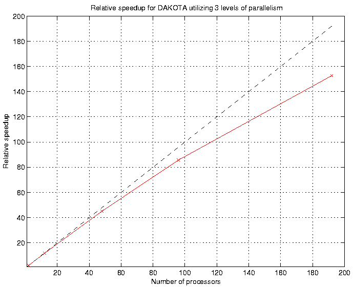
Fig. 61 Relative speedup for Dakota utilizing three levels of parallelism
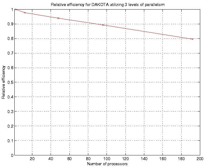
Fig. 62 Relative efficiency for Dakota utilizing three levels of parallelism
Asynchronous Local Parallelism
In most cases, the use of asynchronous local parallelism is the termination point for multilevel parallelism, in that any level of parallelism lower than an asynchronous local level will be serialized (see discussion in the following section Hybrid Parallelism). The exception to this rule is reforking of forked processes for concurrent analyses within forked evaluations. In this case, a new process is created using fork for one of several concurrent evaluations; however, the new process is not replaced immediately using exec. Rather, the new process is reforked to create additional child processes for executing concurrent analyses within each concurrent evaluation process. This capability is not supported by system calls and provides one of the key advantages to using fork over system.
Message Passing Parallelism
Partitioning of levels
Dakota uses MPI communicators to identify groups of processors. The
global MPI_COMM_WORLD communicator provides the total set of
processors allocated to the Dakota run. MPI_COMM_WORLD can be
partitioned into new intra-communicators which each define a set of
processors to be used for a multiprocessor server. Each of these servers
may be further partitioned to nest one level of parallelism within the
next. At the lowest parallelism level, these intra-communicators can be
passed into a simulation for use as the simulation’s computational
context, provided that the simulation has been designed, or can be
modified, to be modular on a communicator (i.e., it does not assume
ownership of MPI_COMM_WORLD). New intra-communicators are created
with the MPI_Comm_split routine, and in order to send messages
between these intra-communicators, new inter-communicators are created
with calls to MPI_Intercomm_create.
Multiple parallel configurations (containing a set of communicator partitions) are allocated for use in studies with multiple iterators and models (e.g., 16 servers of 64 processors each could be used for iteration on a lower fidelity model, followed by two servers of 512 processors each for subsequent iteration on a higher fidelity model), and can be alternated at run time. Each of the parallel configurations are allocated at object construction time and are reported at the beginning of the Dakota output.
Each tier within Dakota’s nested parallelism hierarchy can use the
dedicated master and peer partition approaches described above in the
Partitioning section. To recursively
partition the subcommunicators of Fig. 60,
COMM1/2/3 in the dedicated master or peer partition case would be
further subdivided using the appropriate partitioning model for the next
lower level of parallelism.
Scheduling within levels
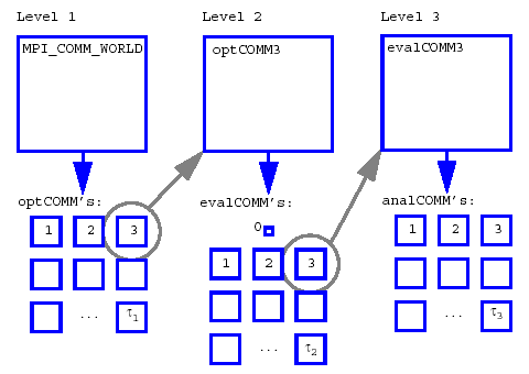
Fig. 63 Recursive partitioning for nested parallelism.
Dakota is designed to allow the freedom to configure each parallelism level with either the dedicated master partition/dynamic scheduling combination or the peer partition/static scheduling combination. In addition, the iterator-evaluation level supports a peer partition/dynamic scheduling option, and certain external libraries may provide custom options.
As an example, Fig. 63 shows a case in which a branch and
bound meta-iterator employs peer partition/distributed scheduling at
level 1, each optimizer partition employs concurrent function
evaluations in a dedicated master partition/dynamic scheduling model at
level 2, and each function evaluation partition employs concurrent
multiprocessor analyses in a peer partition/static scheduling model at
level 3. In this case, MPI_COMM_WORLD is subdivided into
\(optCOMM1/2/3/.../\tau_{1}\), each \(optCOMM\) is further subdivided
into \(evalCOMM0\) (master) and \(evalCOMM1/2/3/.../\tau_{2}\) (slaves),
and each slave \(evalCOMM\) is further subdivided into
\(analysisCOMM1/2/3/.../\tau_{3}\). Logic for selecting the \(\tau_i\)
that maximize overall efficiency is discussed
in [EHSvanBWaanders00].
Hybrid Parallelism
Hybrid parallelism approaches can take several forms when used in the multilevel parallel context. A conceptual boundary can be considered to exist for which all parallelism above the boundary is managed internally using message-passing and all parallelism below the boundary is managed externally using asynchronous local approaches. Hybrid parallelism approaches can then be categorized based on whether this boundary between internal and external management occurs within a parallelism level (intra-level) or between two parallelism levels (inter-level). In the intra-level case, the jobs for the parallelism level containing the boundary are scheduled using a hybrid scheduler, in which a capacity multiplier is used for the number of jobs to assign to each server. Each server is then responsible for concurrently executing its capacity of jobs using an asynchronous local approach. In the inter-level case, one level of parallelism manages its parallelism internally using a message-passing approach and the next lower level of parallelism manages its parallelism externally using an asynchronous local approach. That is, the jobs for the higher level of parallelism are scheduled using a standard message-passing scheduler, in which a single job is assigned to each server. However, each of these jobs has multiple components, as managed by the next lower level of parallelism, and each server is responsible for executing these sub-components concurrently using an asynchronous local approach.
For example, consider a multiprocessor Dakota run which involves an iterator scheduling a set of concurrent function evaluations across a cluster of SMPs. A hybrid parallelism approach will be applied in which message-passing parallelism is used between SMPs and asynchronous local parallelism is used within each SMP. In the hybrid intra-level case, multiple function evaluations would be scheduled to each SMP, as dictated by the capacity of the SMPs, and each SMP would manage its own set of concurrent function evaluations using an asynchronous local approach. Any lower levels of parallelism would be serialized. In the hybrid inter-level case, the function evaluations would be scheduled one per SMP, and the analysis components within each of these evaluations would be executed concurrently using asynchronous local approaches within the SMP. Thus, the distinction can be viewed as whether the concurrent jobs on each server in Fig. 59 reflect the same level of parallelism as that being scheduled by the master (intra-level) or one level of parallelism below that being scheduled by the master (inter-level).
Capability Summary
Table 14 shows a matrix of the supported job
management approaches for each of the parallelism levels, with supported
simulation interfaces and synchronization approaches shown in
parentheses. The concurrent iterator and multiprocessor analysis
parallelism levels can only be managed with message-passing approaches.
In the former case, this is due to the fact that a separate process or
thread for an iterator is not currently supported. The latter case
reflects a finer point on the definition of external parallelism
management. While a multiprocessor analysis can most certainly be
launched (e.g., using mpirun/yod) from one of Dakota’s analysis
drivers, resulting in a parallel analysis external to Dakota (which is
consistent with asynchronous local and hybrid approaches), this
parallelism is not visible to Dakota and therefore does not qualify as
parallelism that Dakota manages (and therefore is not included in
Table 14). The concurrent evaluation and
analysis levels can be managed either with message-passing, asynchronous
local, or hybrid techniques, with the exceptions that the direct
interface does not support asynchronous operations (asynchronous local
or hybrid) at either of these levels and the system call interface does
not support asynchronous operations (asynchronous local or hybrid) at
the concurrent analysis level. The direct interface restrictions are
present since multithreading in not yet supported and the system call
interface restrictions result from the inability to manage concurrent
analyses within a nonblocking function evaluation system call. Finally,
nonblocking synchronization is only supported at the concurrent function
evaluation level, although it spans asynchronous local, message passing,
and hybrid parallelism options.
Parallelism Level |
Asynchronous Local |
Message Passing |
Hybrid |
|---|---|---|---|
concurrent iterators within a meta-iterator or nested model |
X (blocking synch) |
||
concurrent function evaluations within an iterator |
X (system, fork) (blocking, nonblocking) |
X (system, fork, direct) (blocking, nonblocking) |
X (system, fork) (blocking, nonblocking) |
concurrent analyses within a function evaluation |
X (fork only) (blocking synch) |
X (system, fork, direct) (blocking synch) |
X (fork only) (blocking synch) |
fine-grained parallel analysis |
X |
Running a Parallel Dakota Job
Single-level parallelism provides a few examples of serial and parallel execution of Dakota using asynchronous local, message passing, and hybrid approaches to single-level parallelism. The following sections provides a more complete discussion of the parallel execution syntax and available specification controls.
Single-processor execution
The command for running Dakota on a single-processor and exploiting asynchronous local parallelism is the same as for running Dakota on a single-processor for a serial study, e.g.:
dakota -i dakota.in > dakota.out
See Dakota Beginner’s tutorial for additional information on single-processor command syntax.
Multiprocessor execution
Running a Dakota job on multiple processors requires the use of an
executable loading facility such as mpirun, mpiexec, poe, or
yod. On a network of workstations, the mpirun script is commonly
used to initiate a parallel Dakota job, e.g.:
mpirun -np 12 dakota -i dakota.in > dakota.out
mpirun -machinefile machines -np 12 dakota -i dakota.in > dakota.out
where both examples specify the use of 12 processors, the former selecting them from a default system resources file and the latter specifying particular machines in a machine file (see [GL96] for details).
On a massively parallel computer, the familiar mpirun/mpiexec options may be replaced with other launch scripts as dictated by the particular software stack, e.g.:
yod -sz 512 dakota -i dakota.in > dakota.out
In each of these cases, MPI command line arguments are used by MPI
(extracted first in the call to MPI_Init) and Dakota command line
arguments are used by Dakota (extracted second by Dakota’s command line
handler).
Finally, when running on computer resources that employ NQS/PBS batch
schedulers, the single-processor dakota command syntax or the
multiprocessor mpirun command syntax might be contained within an
executable script file which is submitted to the batch queue. For
example, a command
qsub -l size=512 run_dakota
could be submitted to a PBS queue for execution. The NQS syntax is similar:
qsub -q snl -lP 512 -lT 6:00:00 run_dakota
These commands allocate 512 compute nodes for the study, and execute the
run_dakota
script on a service node. If this script contains a single-processor
dakota command, then Dakota will execute on a single service node
from which it can launch parallel simulations into the compute nodes
using analysis drivers that contain yod commands (any yod
executions occurring at any level underneath the run_dakota
script are mapped to
the 512 compute node allocation). If the script submitted to qsub
contains a multiprocessor mpirun command, then Dakota will execute
across multiple service nodes so that it can spread the application load
in either a message-passing or hybrid parallelism approach. Again,
analysis drivers containing yod commands would be responsible for
utilizing the 512 compute nodes. And, finally, if the script submitted
to qsub contains a yod of the dakota executable, then Dakota
will execute directly on the compute nodes and manage all of the
parallelism internally (note that a yod of this type without a
qsub would be mapped to the interactive partition, rather than to
the batch partition).
Not all supercomputers employ the same model for service/compute
partitions or provide the same support for tiling of concurrent
multiprocessor simulations within a single NQS/PBS allocation. For this
reason, templates for parallel job configuration are being catalogued
within dakota/share/dakota/examples/parallelism
(in the software distributions) that are intended to provide
guidance for individual machine idiosyncrasies.
Dakota relies on hints from the runtime environment and command line arguments to detect when it has been launched in parallel. Due to the large number of HPC vendors and MPI implementations, parallel launch is not always detected properly. A parallel launch is indicated by the status message
Running MPI Dakota executable in parallel on N processors.
which is written to the console near the beginning of the Dakota run.
Beginning with release 6.5, if Dakota incorrectly detects a parallel
launch, automatic detection can be overriden by setting the environment
variable DAKOTA_RUN_PARALLEL. If the first character is set to
1, t, or T, Dakota will configure itself to run in parallel.
If the variable exists but is set to anything else, Dakota will
configure itself to run in serial mode.
Specifying Parallelism
Given an allotment of processors, Dakota contains logic based on the theoretical work in [EHSvanBWaanders00] to automatically determine an efficient parallel configuration, consisting of partitioning and scheduling selections for each of the parallelism levels. This logic accounts for problem size, the concurrency supported by particular iterative algorithms, and any user inputs or overrides.
Concurrency is pushed up for most parallelism levels. That is, available
processors will be assigned to concurrency at the higher parallelism
levels first as we partition from the top down. If more processors are
available than needed for concurrency at a level, then the server size
is increased to support concurrency in the next lower level of
parallelism. This process is continued until all available processors
have been assigned. These assignments can be overridden by the user by
specifying a number of servers, processors per server, or both, for the
concurrent iterator, evaluation, and analysis parallelism levels. For
example, if it is desired to parallelize concurrent analyses within each
function evaluation, then an evaluation_servers
override would serialize the concurrent function evaluations level and
ensure processor availability for concurrent analyses.
The exception to this push up of concurrency occurs for concurrent-iterator parallelism levels, since iterator executions tend to have high variability in duration whenever they utilize feedback of results. For these levels, concurrency is pushed down since it is generally best to serialize the levels with the highest job variation and exploit concurrency elsewhere.
Partition type (master or peer) may also be specified for each level, and peer scheduling type (dynamic or static) may be specified at the level of evaluation concurrency. However, these selections may be overridden by Dakota if they are inconsistent with the number of user-requested servers, processors per server, and available processors.
In the following sections, the user inputs and overrides are described, followed by specification examples for single and multi-processor Dakota executions.
The interface specification
Specifying parallelism within an interface can involve the use of the
asynchronous, evaluation_concurrency,
and asynchronous, analysis_concurrency
keywords to specify concurrency local to a processor (i.e., asynchronous
local parallelism). This specification has dual uses:
When running Dakota on a single-processor, the
asynchronouskeyword specifies the use of asynchronous invocations local to the processor (these jobs then rely on external means to be allocated to other processors). The default behavior is to simultaneously launch all function evaluations available from the iterator as well as all available analyses within each function evaluation. In some cases, the default behavior can overload a machine or violate a usage policy, resulting in the need to limit the number of concurrent jobs using theevaluation_concurrencyandanalysis_concurrencyspecifications.When executing Dakota across multiple processors and managing jobs with a message-passing scheduler, the
asynchronouskeyword specifies the use of asynchronous invocations local to each server processor, resulting in a hybrid parallelism approach. In this case, the default behavior is one job per server, which must be overridden with anevaluation_concurrencyspecification and/or ananalysis_concurrencyspecification. When a hybrid parallelism approach is specified, the capacity of the servers (used in the automatic configuration logic) is defined as the number of servers times the number of asynchronous jobs per server.
In both cases, the scheduling of local evaluations is dynamic by
default, but may be explicitly selected or overriden using
local_evaluation_scheduling dynamic
static
In addition, evaluation_servers, processors_per_evaluation,
and evaluation_scheduling keywords can be used to
override the automatic parallel configuration for concurrent function
evaluations. Evaluation scheduling may be selected to be
master or peer,
where the latter must be further specified to be
dynamic or static.
To override the automatic parallelism configuration for concurrent
analyses, the analysis_servers and
analysis_scheduling keywords
may be specified, and the processors_per_analysis
keyword can be used to override the automatic parallelism configuration
for the size of multiprocessor analyses used in a direct function simulation
interface. Scheduling options for this level include
master or
peer, where
the latter is static (no dynamic peer option supported).
The meta-iterator and nested model specifications
To specify concurrency in sub-iterator executions within meta-iterators
(such as sequential) and nested models (such as
sub_method_pointer), the iterator_servers,
processors_per_iterator, and iterator_scheduling keywords are used to
override the automatic parallelism configuration. For this level, the available
scheduling options are master or peer, where the latter is static
(no dynamic peer option supported). See the method and model commands specification
in the Keyword Reference for additional
details.
Single-processor Dakota specification
Specifying a single-processor Dakota job that exploits parallelism
through asynchronous local approaches (see
Fig. 59a) requires inclusion of the
asynchronous keyword in the interface specification.
Once the input file is defined, single-processor Dakota jobs are executed
using the command syntax described previously in
Single-processor execution.
Example 1
For example, the following specification runs an NPSOL optimization which will perform asynchronous finite differencing:
method,
        npsol_sqp

variables,
        continuous_design = 5
          initial_point  0.2  0.05 0.08 0.2  0.2
          lower_bounds   0.15 0.02 0.05 0.1  0.1
          upper_bounds   2.0  2.0  2.0  2.0  2.0

interface,
        system,
          asynchronous
          analysis_drivers = 'text_book'

responses,
        num_objective_functions = 1
        num_nonlinear_inequality_constraints = 2
        numerical_gradients
          interval_type central
          method_source dakota
          fd_gradient_step_size = 1.e-4
        no_hessians
Note that method_source dakota
selects Dakota’s internal finite differencing routine so that the
concurrency in finite difference offsets can be exploited. In this case,
central differencing has been selected and 11 function evaluations (one
at the current point plus two offsets in each of five variables) can be
performed simultaneously for each NPSOL response request. These 11
evaluations will be launched with system calls in the background and
presumably assigned to additional processors through the operating system of
a multiprocessor compute server or other comparable method. The concurrency
specification may be included if it is necessary to limit the maximum number
of simultaneous evaluations. For example, if a maximum of six compute processors
were available, the command
evaluation_concurrency = 6
could be added to the asynchronous specification within the
interface keyword from the preceding example.
Example 2
If, in addition, multiple analyses can be executed concurrently within a function evaluation (e.g., from multiple load cases or disciplinary analyses that must be evaluated to compute the response data set), then an input specification similar to the following could be used:
method,
        npsol_sqp

variables,
        continuous_design = 5
          initial_point  0.2  0.05 0.08 0.2  0.2
          lower_bounds   0.15 0.02 0.05 0.1  0.1
          upper_bounds   2.0  2.0  2.0  2.0  2.0

interface,
        fork
          asynchronous
            evaluation_concurrency = 6
            analysis_concurrency = 3
          analysis_drivers = 'text_book1' 'text_book2' 'text_book3'

responses,
        num_objective_functions = 1
        num_nonlinear_inequality_constraints = 2
        numerical_gradients
          method_source dakota
          interval_type central
          fd_gradient_step_size = 1.e-4
        no_hessians
In this case, the default concurrency with just an asynchronous
specification would be all 11 function evaluations and all 3 analyses,
which can be limited by the and specifications. The input file above
limits the function evaluation concurrency, but not the analysis
concurrency (a specification of 3 is the default in this case and could
be omitted). Changing the input to
evaluation_concurrency = 1
would serialize the function evaluations, and changing the input to
analysis_concurrency = 1
would serialize the analyses.
Multiprocessor Dakota specification
In multiprocessor executions, server evaluations are synchronous
(Fig. 59a) by default and the
asynchronous keyword is only used if a hybrid parallelism approach
(Fig. 59c) is desired. Multiprocessor
Dakota jobs are executed using the command syntax described previously
in Multiprocessor execution
Example 3
To run Example 1 using a message-passing approach, the asynchronous
keyword would be removed (since the servers will execute their
evaluations synchronously), resulting in the following interface
specification:
interface,
        system,
          analysis_drivers = 'text_book'
Running Dakota on 4 processors (syntax:
mpirun -np 4 dakota -i dakota.in) would result in the following
parallel configuration report from the Dakota output:
-----------------------------------------------------------------------------
Dakota parallel configuration:

Level                   num_servers    procs_per_server    partition
-----                   -----------    ----------------    ---------
concurrent evaluations       4                1            peer
concurrent analyses          1                1            peer
multiprocessor analysis      1               N/A           N/A

Total parallelism levels =   1 (1 dakota, 0 analysis)
-----------------------------------------------------------------------------
In this case, a peer partition and dynamic scheduling algorithm are automatically selected for the concurrent evaluations. If a dedicated master is desired instead, then this logic could be overriden by adding:
interface,
        system,
          evaluation_scheduling master
          analysis_drivers = 'text_book'
Running Dakota again on 4 processors (syntax:
mpirun -np 4 dakota -i dakota.in) would now result in this parallel
configuration report:
-----------------------------------------------------------------------------
Dakota parallel configuration:

Level                   num_servers    procs_per_server    partition
-----                   -----------    ----------------    ---------
concurrent evaluations       3                1            ded. master
concurrent analyses          1                1            peer
multiprocessor analysis      1               N/A           N/A

Total parallelism levels =   1 (1 dakota, 0 analysis)
-----------------------------------------------------------------------------
Now the 11 jobs will be dynamically distributed among 3 slave servers, under the control of 1 dedicated master.
As a related example, consider the case where each of the workstations
used in the parallel execution has multiple processors. In this case, a
hybrid parallelism approach which combines message-passing parallelism
with asynchronous local parallelism (see
Fig. 59c) would be a good choice. To
specify hybrid parallelism, one uses the same asynchronous
specification as was used for the single-processor examples, e.g.:
interface,
         system
           asynchronous evaluation_concurrency = 3
           analysis_drivers = `text_book'
With 3 function evaluations concurrent on each server, the capacity of a
4 processor Dakota execution (syntax:
mpirun -np 4 dakota -i dakota.in) has increased to 12 evaluations.
Since all 11 jobs can now be scheduled in a single pass, a peer static
scheduler is sufficient.
-----------------------------------------------------------------------------
Dakota parallel configuration:

Level                   num_servers    procs_per_server    partition
-----                   -----------    ----------------    ---------
concurrent evaluations       4                1            peer
concurrent analyses          1                1            peer
multiprocessor analysis      1               N/A           N/A

Total parallelism levels =   1
-----------------------------------------------------------------------------
Example 4
To run Example 2 using a message-passing approach, the asynchronous
specification is again removed:
interface,
         fork
           analysis_drivers = `text_book1' `text_book2' `text_book3'
Running this example on 6 processors (syntax:
mpirun -np 6 dakota -i dakota.in) would result in the following
parallel configuration report:
-----------------------------------------------------------------------------
Dakota parallel configuration:

Level                   num_servers    procs_per_server    partition
-----                   -----------    ----------------    ---------
concurrent evaluations       6                1            peer
concurrent analyses          1                1            peer
multiprocessor analysis      1               N/A           N/A

Total parallelism levels =   1
-----------------------------------------------------------------------------
in which all of the processors have been assigned to support evaluation concurrency due to the “push up” automatic configuration logic. To assign some of the available processors to the concurrent analysis level, the following input could be used:
interface,
         fork
           analysis_drivers = `text_book1' `text_book2' `text_book3'
           evaluation_scheduling peer static
           evaluation_servers = 2
which results in the following 2-level parallel configuration:
-----------------------------------------------------------------------------
Dakota parallel configuration:

Level                   num_servers    procs_per_server    partition
-----                   -----------    ----------------    ---------
concurrent evaluations       2                3            peer
concurrent analyses          3                1            peer
multiprocessor analysis      1               N/A           N/A

Total parallelism levels =   2
-----------------------------------------------------------------------------
The six processors available have been split into two evaluation servers of three processors each, where the three processors in each evaluation server manage the three analyses, one per processor. Note that without the scheduling override, a dedicated master partition at the evaluation level would have been chosen automatically, dividing the six available processors into one evaluation server with three processors and another with two.
Next, consider the following 3-level parallel case, in which
text_book1, text_book2, and text_book3
from the previous examples now execute on two processors each. In this
case, the processors_per_analysis
keyword is added and the fork interface
is changed to a direct interface since the fine-grained
parallelism of the three simulations is managed internally:
interface,
         direct
           analysis_drivers = `text_book1' `text_book2' `text_book3'
           evaluation_scheduling peer static
           evaluation_servers = 2
           processors_per_analysis = 2
This results in the following parallel configuration for a 12
processor Dakota run (syntax: mpirun -np 12 dakota -i dakota.in):
-----------------------------------------------------------------------------
Dakota parallel configuration:

Level                   num_servers    procs_per_server    partition
-----                   -----------    ----------------    ---------
concurrent evaluations       2                6            peer
concurrent analyses          3                2            peer
multiprocessor analysis      2               N/A           N/A

Total parallelism levels =   3 (2 dakota, 1 analysis)
-----------------------------------------------------------------------------
An important point to recognize is that, since each of the parallel configuration inputs has been tied to the interface specification up to this point, these parallel configurations can be reallocated for each interface in a multi-iterator/multi-model study. For example, a Dakota execution on 40 processors might involve the following two interface specifications:
interface,
        direct,
          id_interface = 'COARSE'
          analysis_driver = 'sim1'
          evaluation_scheduling peer dynamic
          processors_per_analysis = 5

interface,
        direct,
          id_interface = 'FINE'
          analysis_driver = 'sim2'
          evaluation_scheduling peer dynamic
          processors_per_analysis = 10
for which the coarse model would employ 8 evaluation servers of 5 processors each and the fine model would employ 4 evaluation servers of 10 processors each.
Next, consider the following 4-level parallel case that employs the
Pareto set optimization meta-iterator. In this case,
iterator_servers and
iterator_scheduling peer
requests are included in the method specification:
method,
         pareto_set
           iterator_servers = 2
           iterator_scheduling peer
           opt_method_pointer = 'NLP'
           random_weight_sets = 4
Adding this pareto_set method specification to the input file from
the previous 12 processor example results in the following parallel
configuration for a 24 processor Dakota run
(syntax: mpirun -np 24 dakota -i dakota.in):
-----------------------------------------------------------------------------
Dakota parallel configuration:

Level                   num_servers    procs_per_server    partition
-----                   -----------    ----------------    ---------
concurrent iterators         2               12            peer
concurrent evaluations       2                6            peer
concurrent analyses          3                2            peer
multiprocessor analysis      2               N/A           N/A

Total parallelism levels =   4 (3 dakota, 1 analysis)
-----------------------------------------------------------------------------
Note that for this example, the parallel configuration is written to the
file dakota.out.1 because of the use of concurrent iterators.
Example 5
As a final example, consider a multi-start optimization conducted on 384 processors. A job of this size must be submitted to the batch queue, using syntax similar to:
qsub -q snl -lP 384 -lT 6:00:00 run_dakota
where the run_dakota script appears as
#!/bin/sh
cd /scratch/<some_workdir>
yod -sz 384 dakota -i dakota.in > dakota.out
the interface specifications from the dakota.in input file appears as
interface,
        direct,
          analysis_drivers = 'text_book1' 'text_book2' 'text_book3'
          evaluation_servers = 8
          evaluation_scheduling peer dynamic
          processors_per_analysis = 2
and finally, an additional method section is added
method,
        multi_start
          method_pointer = 'CPS'
          iterator_servers = 8
          random_starts = 8
The resulting parallel configuration is reported as
-----------------------------------------------------------------------------
Dakota parallel configuration:

Level                   num_servers    procs_per_server    partition
-----                   -----------    ----------------    ---------
concurrent iterators         8               48            peer
concurrent evaluations       8                6            peer
concurrent analyses          3                2            peer
multiprocessor analysis      2               N/A           N/A

Total parallelism levels =   4 (3 dakota, 1 analysis)
-----------------------------------------------------------------------------
Since the concurrency at each of the nested levels has a multiplicative effect on the number of processors that can be utilized, it is easy to see how large numbers of processors can be put to effective use in reducing the time to reach a solution, even when, as in this example, the concurrency per level is relatively low.
Application Parallelism Use Cases
This section describes several common use cases for running Dakota on parallel computing clusters with various combinations of Dakota and application parallelism. In three of the four cases addressed, the application launched by Dakota is assumed MPI-enabled and run as an independent parallel process.
The examples/parallelism/ folder in the Dakota installation
includes examples of the use cases. In all four, Dakota performs a
vector parameter on the textbook test
function. The application executed for serial demonstration is the text_book
example driver, and for parallel execution, a modified version named
text_book_simple_par. Both are located in Dakota’s share/dakota/test/
folder. Dakota uses its fork interface to launch interface scripts
written either in Bash or Python, which include mock pre-processing to
prepare application input, application execution in serial or
parallel, and post-processing of application results to return to
Dakota.
The combinations of Dakota and application parallelism are summarized in Table 15. In each case, \(M\) denotes the total number of processors (or MPI tasks) allocated and \(N\) denotes the number of processors used by a single application analysis. For most scenarios, Cases 1–3, where Dakota and the application jobs run within a single cluster processor allocation (queued job), are preferred. However for particularly long-running or large jobs, or platforms that not supporting the first scheduling modes, Case 4 may be most appropriate.
Case |
Name |
Dakota |
Application |
Notes |
|---|---|---|---|---|
1 |
Massively Serial |
parallel |
serial |
\(M\) simultaneous application instances, each \(N=1\) processor |
2 |
Sequential Parallel |
serial |
parallel |
1 simultaneous application instance on \(N\) processors |
3 |
Evaluation Tiling |
serial |
parallel |
\(M/N\) simultaneous \(N\) processor jobs |
4 |
Evaluation Submission |
serial |
parallel |
submit expensive \(N\) processor application jobs to a scheduler (e.g., qsub) |
Relevant example files for each case are included in directories
dakota/share/dakota/examples/parallelism/ with
the Dakota distribution. These typically include a PBS or SLURM job
submission script to launch the Dakota study, a Dakota input file, and
a driver script.
Case 1: Massively Serial — Multiple serial analysis jobs
In this case, Dakota will launch multiple simultaneous single processor
application runs (an embarrassingly parallel model). Dakota is run in
parallel, making this example an elaboration of the message-passing
single-level parallel mode.
Specifically in this example, Dakota is run in parallel with \(M=6\)
processors (pbs_submission):
mpiexec -n 6 dakota dakota_pstudy.in
and will launch \(M\) simultaneous analysis jobs, and as each job completes, another will be launched, until all jobs are complete.
If the analysis is extremely fast, performance may be improved by launching multiple evaluation jobs local to each Dakota MPI process, specifying
asynchronous evaluation_concurrency = [2 or more]
As discussed in Hybrid Parallelism, combining MPI and local (asynchronous) parallelism in this way is an example of hybrid parallelism.
Conversely, if the analysis has large memory requirements, Dakota may be launched on fewer than the total number of available cores, which has the effect of increasing the memory available to each MPI task. This is known as undersubscription. In this case, the simulation may still be able to take advantage of thread-based parallelism technologies such as OpenMP. Users are advised to consult their HPC’s documentation or user support to determine how to control the number of MPI tasks launched per compute node.
Hybrid parallelism is another way to reduce Dakota’s memory footprint. Dakota may be launched in parallel using one MPI task per node and configured to run multiple evaluations concurrently on each node using local parallelism. Suppose it is desired to run 160 concurrent evaluations, and the compute nodes each have 16 processors. The job script should reserve 10 nodes, assign one MPI task per node, and to run Dakota using 10 tasks. The interface section of the Dakota input file should contain:
asynchronous evaluation_concurrency = 16
Note: The MPI standard does not support nested calls to MPI_Init.
Although some MPI implementations are tolerant of nested calls and work
as naively expected, it is not possible generally to launch an
MPI-enabled user simulation in parallel beneath Dakota running in
parallel. This restriction includes launching parallelized user
simulations on one core (i.e. mpiexec -n 1).
Case 2: Sequential Parallel — One parallel analysis job at a time
This case is relevant for multi-processor analysis jobs, typically where the analysis is expensive (i.e., is long-running or sufficient processors are not available to run more than one simultaneous analysis). Note that for extremely long-running parallel jobs, Case 4 (Evaluation Submission) below may be more appropriate.
In this case, Dakota runs in serial
dakota dakota_pstudy.in
and the driver script launches the application with mpiexec -n K,
where \(K \leq M\), to launch the application code within the
processor allocation:
mpiexec -n 6 text_book_par application.in application.out
Case 3: Evaluation Tiling — Multiple simultaneous parallel analysis jobs
In this case, the nodes or processors (or MPI tasks) of a single job are partitioned into equally-sized tiles. The number of MPI tasks in each tile is \(N\), the number needed to run the parallel application, and so there are a total of \(M/N\) tiles, where \(M\) is the total number of MPI tasks in the allocation. Dakota, which is run serially by the job script, asynchronously launches evaluations, each of which runs a parallel application on an available tile.
It is up to the user to ensure consistency among the number of nodes in
the allocation, the number of processors (or MPI tasks) per node,
Dakota’s evaluation_concurrency, and the number of processors (or
MPI tasks) per parallel application run. For instance, suppose it is
desired to perform 10 concurrent runs of a parallel application, each
requiring 32 processors. The compute nodes each have 16 processors. The
job script must reserve 2 nodes per application run (\(32/16\)) for
a total of \(2 \cdot 10 = 20\) nodes. Dakota’s
evaluation_concurrency must be set to 10.
Under ideal circumstances, as Dakota concurrently launches evaluations
of the user’s parallel application, the cluster workload manager (e.g.
SLURM, PBS) performs load balancing and ensures that the runs “land” on
idle resources. In this situation, the Dakota-application interface
script is relatively simple; in the execution phase, the application is
run using the appropriate parallel launcher (e.g. srun), specifying
the number of MPI tasks to use.
However, if load balancing is not automatically handled by the workload manager, and the user does nothing to manage tiling, then all the evaluations may land on the first few nodes, leaving the rest idle and severly degrading performance. Clearly, care must be taken to ensure that evaluations are tiled correctly.
Whether correct evaluation tiling occurs automatically can depend intimately on how the HPC adminstrators configured the workload manager and MPI. Users are advised to perform small-scale experiments to determine whether performance is as expected, and/or to contact their system administrator for guidance.
Dakota provides a few examples and tools to help users orchestrate placement of parallel applications on available resources when the resource manager does not. They are explained in the following sections.
A related consideration is the memory usage of Dakota itself. If the user’s application is memory intensive, it may be desirable to reserve a node or a portion of a node for Dakota to prevent it from degrading the performance of evaluations. It is necessary in this case to determine where the job script, and hence Dakota, is run. Consulting the workload manager’s documenation or the HPC’s system administrator is advised.
Mpiexec server mode
Mpiexec (http://www.osc.edu/ pw/mpiexec/) works in concert with MPICH
implementations, extending mpirun to run jobs in a PBS environment with
additional features. It offers a background server option which can be
used to tile multiple MPI jobs within a single parallel resource
allocation. (Note that with MPICH, there is a difference between
mpirun and mpiexec, unlike with OpenMPI, where both are
typically aliases for orterun.) See the example in
Case3-EvaluationTiling/MPICH.
In this case, an mpiexec server process is started and backgrounded
to service application requests for processors; Dakota runs in serial
(pbs_submission):
mpiexec -server &

dakota dakota_pstudy.in
and asynchronously launches \(M/N=3\) evaluations (dakota_pstudy.in):
interface
  fork
    asynchronous evaluation_concurrency = 3
    analysis_driver = 'text_book_par_driver'
The simulator script calls mpiexec -n 2 to run the analysis in
parallel and the mpiexec server assigns a subset of the available
processors to the particular MPI task (text_book_par):
mpiexec -n 2 text_book_simple_par application.in application.out
An error will result if more application tasks are launched than the processor allocation permits. An error may result if the application does not exit cleanly. At present similar capability is not supported by OpenMPI, although a daemon mode similar to Mpiexec has been proposed.
Relative node scheduling
This Evaluation Tiling variant uses OpenMPI 1.3.3 or newer. It leverages
Dakota’s option together with integer arithmetic to schedule each
evaluation on the right subset of the processor allocation. A Bash-based
example is provided in Case3-EvaluationTiling/OpenMPI.
Similar approaches work with some AIX/POE installations as well.
The mpitile utility, released with Dakota 6.6, transparently manages
construction of relative node lists when using the OpenMPI command
mpirun and the SLURM workload manager. mpitile resides in the
Dakota bin/ folder and is a wrapper for mpirun. It uses a file locking
mechanism to support dynamic scheduling of evaluations but also has a
–static option. Using the –dedicated-master option, either an
entire NODE or a TILE can be reserved for Dakota. Running
mpitile with the –help option provides a basic description of
its options. The script text_book_mpitile_dynamic.sh in the
OpenMPI example folder demonstrates usage of mpitile.
mpitile is based on the Python module
dakota.interfacing.parallel, also released with Dakota 6.6.
Interface scripts written in Python may benefit from using its API
directly. An example is located at
Case3-EvaluationTiling/OpenMPI/text_book_di_dynamic.py. The
dakota Python package is located in
dakota/share/dakota/Python/, which users should add to the
environment variable PYTHONPATH.
Machinefile management
This Evaluation Tiling variant applies when the application must be
compiled with OpenMPI or another MPI implementation that does not
support a server mode for job tiling, but does support the use of
machine files specifying the resources on which to run the application
job. A set of scripts are used to manage the partitioning of the
\(M\) processor allocation into tiles contain \(N\) processors.
Each tile has an associated machines file consisting of a unique subset
of the assigned resources. Note that this will not work with early
OpenMPI versions with some resource managers (e.g., OpenMPI 1.2 with
Torque), where machinefiles, even if a proper subset of
$PBS_NODEFILE, are ignored. This will however work with OpenMPI 1.3
and newer. See the example in Case3-EvaluationTiling/MachinefileMgmt.
In this case the pbs_submission script defines variables specifying
how to create a separate node file for each job and sets up a set of
nodefiles for use by each evaluation. As when using relative node lists,
Dakota runs in serial and uses asynchronous evaluation concurrency to
launch the jobs. The interface script text_book_par_driver
contains logic to lock a node file
for the application run and return it when complete. As each job
completes, the next is scheduled.
Case 4: Evaluation Submission — Parallel analysis jobs submitted to a queue
This case describes running Dakota to submit parallel jobs to a batch queue. This option is likely only useful when the cost of an individual analysis evaluation is high (such that the job requires far too many processors or hours to run all the evaluations) and there is no feedback to Dakota required to generate subsequent evaluation points. So this scenario is likely more relevant for sensitivity analysis and uncertainty quantification than optimization.
In the first pass, Dakota runs (likely interactively) in serial on a login node or other node capable of job submission:
dakota dakota_pstudy.in
For each evaluation, the simulator script (text_book_par_driver)
will generate a pbs_submission script and submit it to the
scheduler. Dummy results are returned to Dakota which will exit when
all jobs have been scheduled.
In the second pass, when analysis is complete, the analysis driver is
changed to post_process and Dakota is executed on a login node to
collect the results of the study.