Additional Examples

This chapter contains additional examples of available methods being applied to several test problems. The examples are organized by the test problem being used. Many of these examples are also used as code verification tests. The examples are run periodically and the results are checked against known solutions. This ensures that the algorithms are correctly implemented.

Textbook

The two-variable version of the “textbook” test problem provides a nonlinearly constrained optimization test case. It is formulated as:

(1)$$\begin{array}{rl}\mathtt{\text{minimize }}& f=(x_1-1{)}^4+(x_2-1{)}^4\\ \mathtt{\text{subject to }}& g_1=x_1^2-\frac{x_2}{2}\le 0\\ & g_2=x_2^2-\frac{x_1}{2}\le 0\\ & 0.5\le x_1\le 5.8\\ & -2.9\le x_2\le 2.9\end{array}$$

Contours of this test problem are illustrated in Fig. 7, with a close-up view of the feasible region given in Fig. 8.

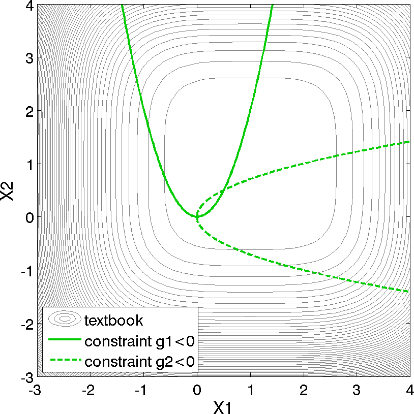
Fig. 7 Contours of the textbook problem on the $[-3,4]\times [-3,4]$ domain with the constrained optimum point $(x_1,x_2)=(0.5,0.5)$. The feasible region lies at the intersection of the two constraints $g_1$ (solid) and $g_2$ (dashed).

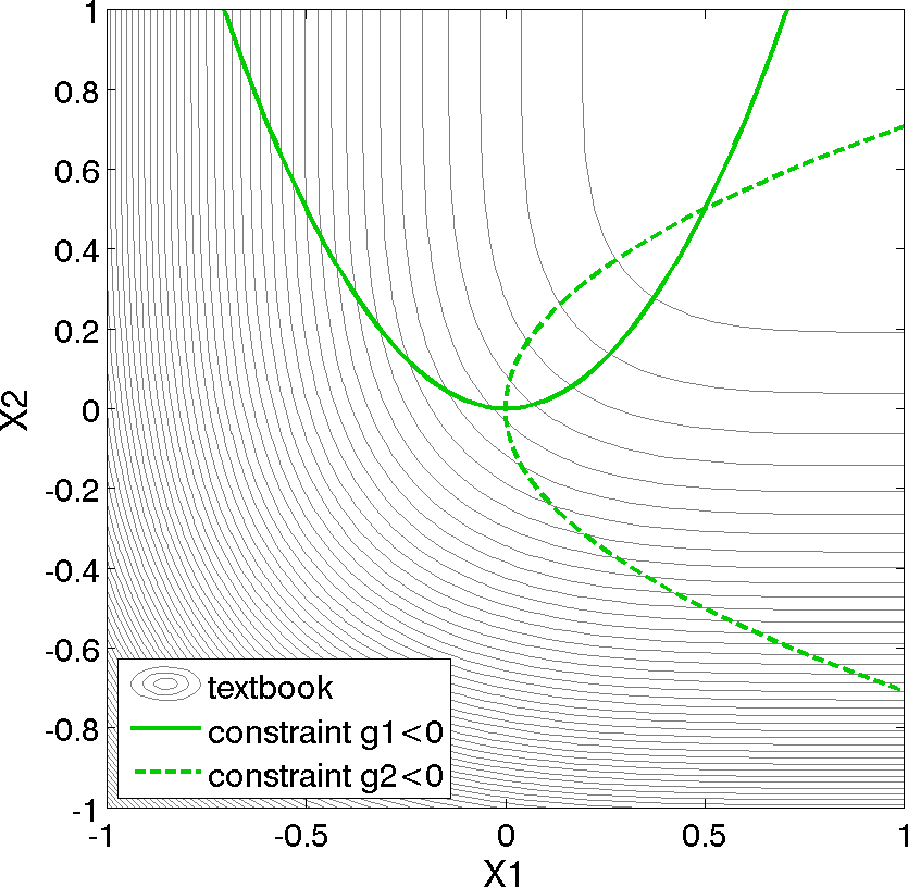
Fig. 8 Contours of the textbook problem zoomed into an area containing the constrained optimum point $(x_1,x_2)=(0.5,0.5)$. The feasible region lies at the intersection of the two constraints $g_1$ (solid) and $g_2$ (dashed).

For the textbook test problem, the unconstrained minimum occurs at $(x_1,x_2)=(1,1)$. However, the inclusion of the constraints moves the minimum to $(x_1,x_2)=(0.5,0.5)$. Equation (1) presents the 2-dimensional form of the textbook problem. An extended formulation is given by

(2)$$\begin{array}{rl}\mathtt{\text{minimize }}& f=\sum _{i=1}^n(x_i-1{)}^4\\ \mathtt{\text{subject to }}& g_1=x_1^2-\frac{x_2}{2}\le 0\\ & g_2=x_2^2-\frac{x_1}{2}\le 0\\ & 0.5\le x_1\le 5.8\\ & -2.9\le x_2\le 2.9\end{array}$$

where $n$ is the number of design variables. The objective function is designed to accommodate an arbitrary number of design variables in order to allow flexible testing of a variety of data sets. Contour plots for the $n=2$ case have been shown previously in Fig. 7.

For the optimization problem given in Equation (2), the unconstrained solution num_nonlinear_inequality_constraints = 0 for two design variables is:

$$\begin{array}{rl}{x}_1& =1.0\\ x_2& =1.0\end{array}$$

with

$$f^{\ast }=0.0$$

The solution for the optimization problem constrained by $g_1$ (num_nonlinear_inequality_constraints = 1) is:

$$\begin{array}{rl}{x}_1& =0.763\\ x_2& =1.16\end{array}$$

with

$$\begin{array}{rl}{f}^{\ast }& =0.00388\\ g_1^{\ast }& =0.0(\mathrm{active})\end{array}$$

The solution for the optimization problem constrained by $g_1$ and $g_2$ (num_nonlinear_inequality_constraints = 2) is:

$$\begin{array}{rl}{x}_1& =0.500\\ x_2& =0.500\end{array}$$

with

$$\begin{array}{rl}{f}^{\ast }& =0.125\\ g_1^{\ast }& =0.0(\mathrm{active})g_2^{\ast }& =0.0(\mathrm{active})\end{array}$$

Note that as constraints are added, the design freedom is restricted (the additional constraints are active at the solution) and an increase in the optimal objective function is observed.

Gradient-based Constrained Optimization

This example demonstrates the use of a gradient-based optimization algorithm on a nonlinearly constrained problem. The Dakota input file for this example is shown in Listing 4. This input file is similar to the input file for the unconstrained gradient-based optimization example involving the Rosenbrock function, seen in Optimization Note the addition of commands in the responses block of the input file that identify the number and type of constraints, along with the upper bounds on these constraints. The commands direct and analysis_driver = ’text_book’ specify that Dakota will use its internal version of the textbook problem.

Listing 4 Textbook gradient-based constrained optimization example: the Dakota input file – see dakota/share/dakota/examples/users/textbook_opt_conmin.in

# Dakota Input File: textbook_opt_conmin.in

environment
  tabular_data
    tabular_data_file = 'textbook_opt_conmin.dat'

method
# dot_mmfd #DOT performs better but may not be available
  conmin_mfd
    max_iterations = 50
    convergence_tolerance = 1e-4

variables
  continuous_design = 2
    initial_point    0.9    1.1
    upper_bounds     5.8    2.9
    lower_bounds     0.5   -2.9
    descriptors      'x1'   'x2'

interface
  analysis_drivers =       'text_book'
    direct

responses
  objective_functions = 1
  nonlinear_inequality_constraints = 2
  descriptors 'f' 'c1' 'c2'
  numerical_gradients
    method_source dakota
    interval_type central
    fd_step_size = 1.e-4
  no_hessians

The conmin_mfd keyword in Listing 4 tells Dakota to use the CONMIN package’s implementation of the Method of Feasible Directions (see Methods for Constrained Problems for more details). A significantly faster alternative is the DOT package’s Modified Method of Feasible Directions, i.e. dot_mmfd (see Methods for Constrained Problems for more details). However, DOT is licensed software that may not be available on a particular system. If it is installed on your system and Dakota has been configured and compiled with HAVE_DOT:BOOL=ON flag, you may use it by commenting out the line with conmin_mfd and uncommenting the line with dot_mmfd.

The results of the optimization example are listed at the end of the output file (see discussion in What should happen). This information shows that the optimizer stopped at the point $(x_1,x_2)=(0.5,0.5)$, where both constraints are approximately satisfied, and where the objective function value is $0.128$. The progress of the optimization algorithm is shown in Fig. 9 where the dots correspond to the end points of each iteration in the algorithm. The starting point is $(x_1,x_2)=(0.9,1.1)$, where both constraints are violated. The optimizer takes a sequence of steps to minimize the objective function while reducing the infeasibility of the constraints. Dakota’s legacy X Windows-based graphics for the optimization are also shown in Fig. 10.

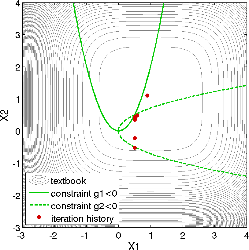
Fig. 9 Textbook gradient-based constrained optimization example: iteration history (iterations marked by solid dots).

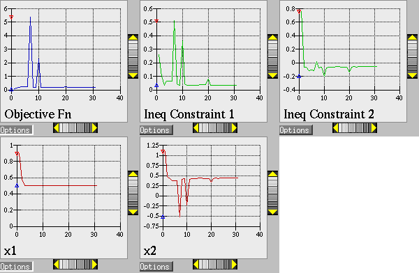
Fig. 10 Textbook gradient-based constrained optimization example: screen capture of the legacy Dakota X Windows-based graphics shows how the objective function was reduced during the search for a feasible design point

Least Squares Optimization

This test problem may also be used to exercise least squares solution methods by modifying the problem formulation to:

(3)$$\mathtt{\text{minimize }}(f{)}^2+(g_1{)}^2+(g_2{)}^2$$

This modification is performed by simply changing the responses specification for the three functions from num_objective_functions = 1 and num_nonlinear_inequality_constraints = 2 to num_least_squares_terms = 3. Note that the two problem formulations are not equivalent and have different solutions.

Note

Another way to exercise the least squares methods which would be equivalent to the optimization formulation would be to select the residual functions to be $(x_i-1{)}^2$. However, this formulation requires modification to dakota_source/test/text_book.cpp and will not be presented here. Equation (3), on the other hand, can use the existing text_book without modification.

Refer to Rosenbrock for an example of minimizing the same objective function using both optimization and least squares approaches.

The solution for the least squares problem given in (3) is:

$$\begin{array}{rl}{x}_1& =0.566\\ x_2& =0.566\end{array}$$

with the residual functions equal to

$$\begin{array}{rl}{f}^{\ast }& =0.0713\\ g_1^{\ast }& =0.0371\\ g_2^{\ast }& =0.0371\end{array}$$

and therefore a sum of squares equal to 0.00783.

This study requires selection of num_least_squares_terms = 3 in the responses specification and selection of either optpp_g_newton, nlssol_sqp, or nl2sol in the method specification.

Rosenbrock

The Rosenbrock function [GMW81] is a well known test problem for optimization algorithms. The standard formulation includes two design variables, and computes a single objective function, while generalizations can support arbitrary many design variables. This problem can also be posed as a least-squares optimization problem with two residuals to be minimized because the objective function is comprised of a sum of squared terms.

Standard Formulation: The standard two-dimensional formulation is

(4)$$\mathtt{\text{minimize }}f(x)=100(x_2-x_1^2{)}^2+(1-x_1{)}^2$$

Surface and contour plots for this function can be seen in Rosenbrock Test Problem. The optimal solution is:

$$\begin{array}{rl}{x}_1& =1.0\\ x_2& =1.0\end{array}$$

with

$$f^{\ast }=0.0$$

A discussion of gradient based optimization to minimize this function is in Optimization

“Extended” Formulation: The formulation in [NJ99], called the “extended Rosenbrock”, is defined by:

(5)$$f=\sum _{i=1}^{n/2}[\alpha (x_{2i}-x_{2i-1}^2{)}^2+(1-x_{2i-1}{)}^2]$$

“Generalized” Formulation: Another n-dimensional formulation was propsed in [Sch87]:

(6)$$f=\sum _{i=1}^{n-1}[100(x_{i+1}-x_i^2{)}^2+(1-x_i{)}^2]$$

A Least-Squares Optimization Formulation: This test problem may also be used to exercise least-squares solution methods by recasting the standard problem formulation into:

(7)$$\mathtt{\text{minimize }}f(x)=(f_1{)}^2+(f_2{)}^2$$

where

(8)$$f_1=10(x_2-x_1^2)$$

and

(9)$$f_2=1-x_1$$

are residual terms.

The included analysis driver can handle both formulations. In the dakota/share/dakota/test directory, the rosenbrock executable (compiled from dakota_source/test/rosenbrock.cpp) checks the number of response functions passed in the parameters file and returns either an objective function (as computed from (4)) for use with optimization methods or two least squares terms (as computed from (8) and (9)) for use with least squares methods. Both cases support analytic gradients of the function set with respect to the design variables. See Listing 1 (standard formulation) and Listing 5 (least squares formulation) for usage examples.

Least-Squares Optimization

Least squares methods are often used for calibration or parameter estimation, that is, to seek parameters maximizing agreement of models with experimental data. The least-squares formulation was described in the previous section.

When using a least-squares approach to minimize a function, each of the least-squares terms $f_1,f_2,\dots$ is driven toward zero. This formulation permits the use of specialized algorithms that can be more efficient than general purpose optimization algorithms. See Nonlinear Least Squares for more detail on the algorithms used for least-squares minimization, as well as a discussion on the types of engineering design problems (e.g., parameter estimation) that can make use of the least-squares approach.

Listing 5 is a listing of the Dakota input file rosen_opt_nls.in. This differs from the input file shown in Rosenbrock gradient-based unconstrained optimization example: the Dakota input file. in several key areas. The responses block of the input file uses the keyword calibration_terms = 2 instead of objective_functions = 1. The method block of the input file shows that the NL2SOL algorithm [DGW81] (nl2sol) is used in this example. (The Gauss-Newton, NL2SOL, and NLSSOL SQP algorithms are currently available for exploiting the special mathematical structure of least squares minimization problems).

Listing 5 Rosenbrock nonlinear least squares example: the Dakota input file – see dakota/share/dakota/examples/users/rosen_opt_nls.in

# Dakota Input File: rosen_opt_nls.in

environment
  tabular_data
    tabular_data_file = 'rosen_opt_nls.dat'

method
  nl2sol
    convergence_tolerance = 1e-4
    max_iterations = 100

model
  single

variables
  continuous_design = 2
    initial_point    -1.2      1.0
    lower_bounds     -2.0     -2.0
    upper_bounds      2.0      2.0
    descriptors       'x1'     "x2"

interface
  analysis_drivers = 'rosenbrock'
    direct

responses
  calibration_terms = 2
  analytic_gradients
  no_hessians

The results at the end of the output file show that the least squares minimization approach has found the same optimum design point, $(x1,x2)=(1.0,1.0)$, as was found using the conventional gradient-based optimization approach. The iteration history of the least squares minimization is shown in Fig. 11, and shows that 14 function evaluations were needed for convergence. In this example the least squares approach required about half the number of function evaluations as did conventional gradient-based optimization. In many cases a good least squares algorithm will converge more rapidly in the vicinity of the solution.

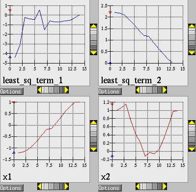
Fig. 11 Rosenbrock nonlinear least squares example: iteration history for least squares terms $f_1$ and $f_2$.

Method Comparison

In comparing the two approaches, one would expect the Gauss-Newton approach to be more efficient since it exploits the special-structure of a least squares objective function and, in this problem, the Gauss-Newton Hessian is a good approximation since the least squares residuals are zero at the solution. From a good initial guess, this expected behavior is clearly demonstrated. Starting from cdv_initial_point = 0.8, 0.7, the optpp_g_newton method converges in only 3 function and gradient evaluations while the optpp_q_newton method requires 27 function and gradient evaluations to achieve similar accuracy. Starting from a poorer initial guess (e.g., cdv_initial_point = -1.2, 1.0), the trend is less obvious since both methods spend several evaluations finding the vicinity of the minimum (total function and gradient evaluations = 45 for optpp_q_newton and 29 for optpp_g_newton). However, once the vicinity is located and the Hessian approximation becomes accurate, convergence is much more rapid with the Gauss-Newton approach.

Shown below is the complete Dakota output for the optpp_g_newton method starting from cdv_initial_point = 0.8, 0.7:

Running MPI executable in serial mode.
Dakota version 6.0 release.
Subversion revision xxxx built May ...
Writing new restart file dakota.rst
gradientType = analytic
hessianType = none

>>>>> Executing environment.

>>>>> Running optpp_g_newton iterator.

------------------------------
Begin Function Evaluation    1
------------------------------
Parameters for function evaluation 1:
                      8.0000000000e-01 x1
                      7.0000000000e-01 x2

rosenbrock /tmp/file4t29aW /tmp/filezGeFpF

Active response data for function evaluation 1:
Active set vector = { 3 3 } Deriv vars vector = { 1 2 }
                      6.0000000000e-01 least_sq_term_1
                      2.0000000000e-01 least_sq_term_2
 [ -1.6000000000e+01  1.0000000000e+01 ] least_sq_term_1 gradient
 [ -1.0000000000e+00  0.0000000000e+00 ] least_sq_term_2 gradient




------------------------------
Begin Function Evaluation    2
------------------------------
Parameters for function evaluation 2:
                      9.9999528206e-01 x1
                      9.5999243139e-01 x2

rosenbrock /tmp/fileSaxQHo /tmp/fileHnU1Z7

Active response data for function evaluation 2:
Active set vector = { 3 3 } Deriv vars vector = { 1 2 }
                     -3.9998132761e-01 least_sq_term_1
                      4.7179363810e-06 least_sq_term_2
 [ -1.9999905641e+01  1.0000000000e+01 ] least_sq_term_1 gradient
 [ -1.0000000000e+00  0.0000000000e+00 ] least_sq_term_2 gradient




------------------------------
Begin Function Evaluation    3
------------------------------
Parameters for function evaluation 3:
                      9.9999904377e-01 x1
                      9.9999808276e-01 x2

rosenbrock /tmp/filedtRtlR /tmp/file3kUVGA

Active response data for function evaluation 3:
Active set vector = { 3 3 } Deriv vars vector = { 1 2 }
                     -4.7950734494e-08 least_sq_term_1
                      9.5622502239e-07 least_sq_term_2
 [ -1.9999980875e+01  1.0000000000e+01 ] least_sq_term_1 gradient
 [ -1.0000000000e+00  0.0000000000e+00 ] least_sq_term_2 gradient




------------------------------
Begin Function Evaluation    4
------------------------------
Parameters for function evaluation 4:
                      9.9999904377e-01 x1
                      9.9999808276e-01 x2

Duplication detected: analysis_drivers not invoked.

Active response data retrieved from database:
Active set vector = { 2 2 } Deriv vars vector = { 1 2 }
 [ -1.9999980875e+01  1.0000000000e+01 ] least_sq_term_1 gradient
 [ -1.0000000000e+00  0.0000000000e+00 ] least_sq_term_2 gradient


<<<<< Function evaluation summary: 4 total (3 new, 1 duplicate)
<<<<< Best parameters          =
                      9.9999904377e-01 x1
                      9.9999808276e-01 x2
<<<<< Best residual norm =  9.5742653315e-07; 0.5 * norm^2 =  4.5833278319e-13
<<<<< Best residual terms      =
                     -4.7950734494e-08
                      9.5622502239e-07
<<<<< Best evaluation ID: 3
Confidence Interval for x1 is [  9.9998687852e-01,  1.0000112090e+00 ]
Confidence Interval for x2 is [  9.9997372187e-01,  1.0000224436e+00 ]

<<<<< Iterator optpp_g_newton completed.
<<<<< Environment execution completed.
Dakota execution time in seconds:
  Total CPU        =       0.01 [parent =   0.017997, child =  -0.007997]
  Total wall clock =  0.0672231

Herbie, Smooth Herbie, and Shubert

Lee, et al. [LGLG11] developed the Herbie function as a 2D test problem for surrogate-based optimization. However, since it is separable and each dimension is identical it is easily generalized to an arbitrary number of dimensions. The generalized (to $M$ dimensions) Herbie function is

$$\mathrm{h}\mathrm{e}\mathrm{r}\mathrm{b}(x)=-\prod _{k=1}^M{w}_{herb}\left(x_k\right)$$

where

$$w_{herb}\left(x_k\right)=\exp (-(x_k-1{)}^2)+\exp (-0.8(x_k+1{)}^2)-0.05\sin \left(8(x_k+0.1)\right).$$

The Herbie function’s high frequency sine component creates a large number of local minima and maxima, making it a significantly more challenging test problem. However, when testing a method’s ability to exploit smoothness in the true response, it is desirable to have a less oscillatory function. For this reason, the “smooth Herbie” test function omits the high frequency sine term but is otherwise identical to the Herbie function. The formula for smooth Herbie is

$$\mathrm{h}\mathrm{e}\mathrm{r}{\mathrm{b}}_{\mathrm{s}\mathrm{m}}(x)=-\prod _{k=1}^M{w}_{sm}\left(x_k\right)$$

where

$$w_{sm}\left(x_k\right)=\exp (-(x_k-1{)}^2)+\exp (-0.8(x_k+1{)}^2).$$

Two dimensional versions of the herbie and smooth_herbie test functions are plotted in Fig. 12.

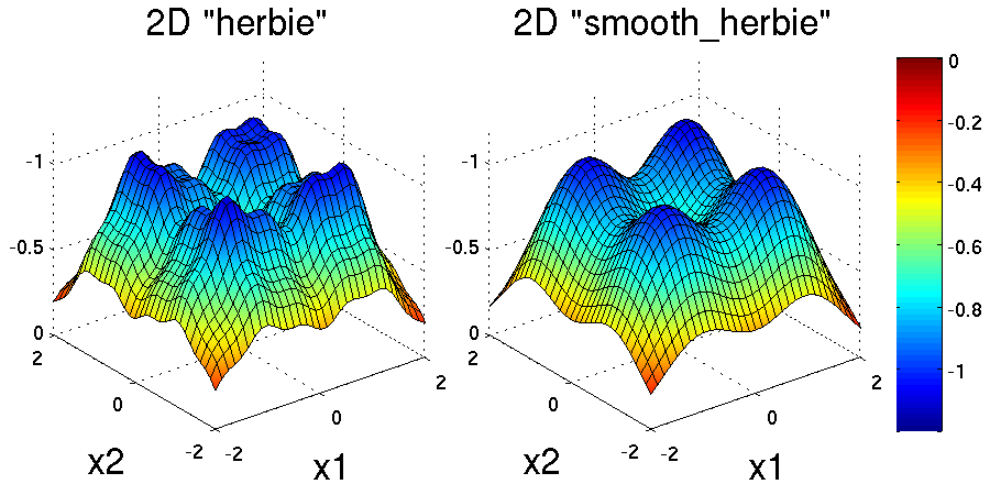
Fig. 12 Plots of the herbie (left) and smooth_herbie (right) test functions in 2 dimensions. They can accept an arbitrary number of inputs. The direction of the z-axis has been reversed (negative is up) to better view the functions’ minima.

Shubert is another separable (and therefore arbitrary dimensional) test function. Its analytical formula is

$$\begin{array}{rl}\mathrm{s}\mathrm{h}\mathrm{u}(x)& =\prod _{k=1}^M{w}_{shu}\left(x_k\right)\\ w_{shu}\left(x_k\right)& =\sum _{i=1}^{5}i\cos ((i+1)x_k+i)\end{array}$$

The 2D version of the shubert function is shown in Fig. 13.

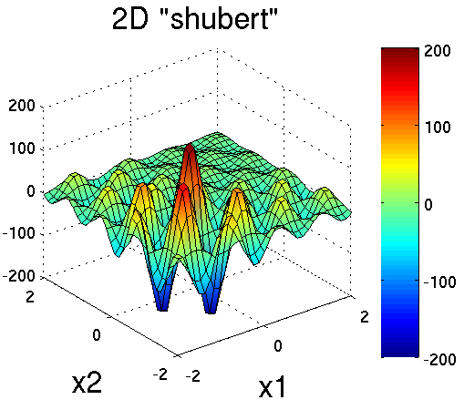
Fig. 13 Plot of the shubert test function in 2 dimensions. It can accept an arbitrary number of inputs.

Efficient Global Optimization

The Dakota input file herbie_shubert_opt_ego.in shows how to use efficient global optimization (EGO) to minimize the 5D version of any of these 3 separable functions. The input file is shown in Listing 6. Note that in the variables section the 5* preceding the values -2.0 and 2.0 for the lower_bounds and upper_bounds, respectively, tells Dakota to repeat them 5 times. The “interesting” region for each of these functions is $-2\le x_k\le 2$ for all dimensions.

Listing 6 Herbie/Shubert examples: the Dakota input file – see dakota/share/dakota/examples/users/herbie_shubert_opt_ego.in

# Dakota Input File: herbie_shubert_opt_ego.in
# Example of using EGO to find the minumum of the 5 dimensional version
# of the abitrary-dimensional/separable 'herbie' OR 'smooth_herbie' OR
# 'shubert' test functions
environment
  tabular_data
    tabular_data_file = 'herbie_shubert_opt_ego.dat'

method
  efficient_global      # EGO Efficient Global Optimization
    initial_samples 50
    seed = 123456

variables
  continuous_design = 5       # 5 dimensions
    lower_bounds      5*-2.0  # use 5 copies of -2.0 for bound
    upper_bounds      5*2.0   # use 5 copies of 2.0 for bound

interface
#  analysis_drivers = 'herbie'       # use this for herbie
  analysis_drivers = 'smooth_herbie' # use this for smooth_herbie
#  analysis_drivers = 'shubert'      # use this for shubert
    direct

responses
  objective_functions = 1
  no_gradients
  no_hessians

Sobol and Ishigami Functions

These functions, documented in [SSHS09], are often used to test sensitivity analysis methods. The Sobol rational function is given by the equation:

$$f(\mathbf{x})=\frac{(x_2+0.5{)}^4}{(x_1+0.5{)}^2}$$

This function is monotonic across each of the inputs. However, there is substantial interaction between $x_1$ and $x_2$ which makes sensitivity analysis difficult. This function in shown in Fig. 14.

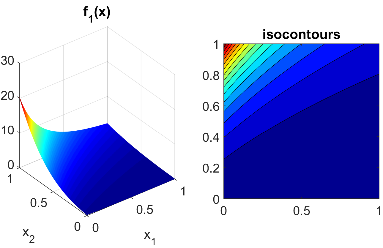
Fig. 14 Plot of the sobol_rational test function in 2 dimensions.

The Ishigami test problem is a smooth $C^{\mathrm{\infty }}$ function:

$$f(\mathbf{x})=\sin (2\pi x_1-\pi )+7{\sin }^2(2\pi x_2-\pi )+0.1(2\pi x_3-\pi {)}^4\sin (2\pi x_1-\pi )$$

where the distributions for $x_1$, $x_2$, and $x_3$ are iid uniform on [0,1]. This function was created as a test for global sensitivity analysis methods, but is challenging for any method based on low-order structured grids (e.g., due to term cancellation at midpoints and bounds). This function in shown in Fig. 15.

Fig. 15 Plot of the sobol_ishigami test function as a function of x1 and x3.

At the opposite end of the smoothness spectrum, Sobol’s g-function is $C^0$ with the absolute value contributing a slope discontinuity at the center of the domain:

$$f(\mathbf{x})=2\prod _{j=1}^5\frac{|4x_j-2|+a_j}{1+a_j};a=[0,1,2,4,8]$$

The distributions for $x_j$ for $j=1,2,3,4,5$ are iid uniform on [0,1]. This function in shown in Fig. 16.

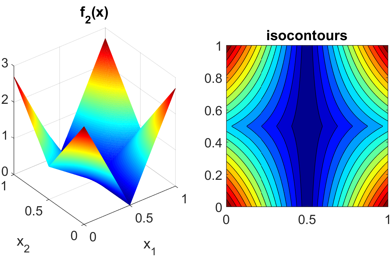
Fig. 16 Plot of the sobol_g_function test function.

Cylinder Head

The cylinder head test problem is stated as:

(10)$$\begin{array}{rl}\mathtt{\text{minimize }}& f=-1(\frac{\mathtt{horsepower}}{250}+\frac{\mathtt{warranty}}{100000})\\ \mathtt{\text{subject to }}& {\sigma }_{max}\le 0.5{\sigma }_{yield}\\ & \mathtt{warranty}\ge 100000\\ & {\mathtt{time}}_{\mathtt{cycle}}\le 60\\ & 1.5\le {\mathtt{d}}_{\mathtt{intake}}\le 2.164\\ & 0.0\le \mathtt{flatness}\le 4.0\end{array}$$

This formulation seeks to simultaneously maximize normalized engine horsepower and engine warranty over variables of valve intake diameter (${\mathtt{d}}_{\mathtt{intake}}$) in inches and overall head flatness ($\mathtt{flatness}$) in thousandths of an inch subject to inequality constraints that the maximum stress cannot exceed half of yield, that warranty must be at least 100000 miles, and that manufacturing cycle time must be less than 60 seconds. Since the constraints involve different scales, they should be nondimensionalized (note: the nonlinear constraint scaling described in Optimization with User-specified or Automatic Scaling can now do this automatically). In addition, they can be converted to the standard 1-sided form $g(\mathbf{x})\le 0$ as follows:

(11)$$\begin{array}{rlr}& & g_1=\frac{2{\sigma }_{\mathtt{max}}}{{\sigma }_{\mathtt{yield}}}-1\le 0\\ & & g_2=1-\frac{\mathtt{warranty}}{100000}\le 0\\ & & g_3=\frac{{\mathtt{time}}_{\mathtt{cycle}}}{60}-1\le 0\end{array}$$

The objective function and constraints are related analytically to the design variables according to the following simple expressions:

(12)$$\begin{array}{rl}\mathtt{warranty}& =100000+15000(4-\mathtt{flatness})\\ {\mathtt{time}}_{\mathtt{cycle}}& =45+4.5(4-\mathtt{flatness}{)}^{1.5}\\ \mathtt{horsepower}& =250+200(\frac{{\mathtt{d}}_{\mathtt{intake}}}{1.833}-1)\\ {\sigma }_{\mathtt{max}}& =750+\frac{1}{({\mathtt{t}}_{\mathtt{wall}}{)}^{2.5}}\\ {\mathtt{t}}_{\mathtt{wall}}& ={\mathtt{offset}}_{\mathtt{intake}}\mathtt{-}{\mathtt{offset}}_{\mathtt{exhaust}}-\frac{({\mathtt{d}}_{\mathtt{intake}}\mathtt{+}{\mathtt{d}}_{\mathtt{exhaust}})}{2}\end{array}$$

where the constants in (11) and (12) assume the following values: ${\sigma }_{\mathtt{yield}}=3000$, ${\mathtt{offset}}_{\mathtt{intake}}=3.25$, ${\mathtt{offset}}_{\mathtt{exhaust}}=1.34$, and ${\mathtt{d}}_{\mathtt{exhaust}}=1.556$.

Constrained Gradient Based Optimization

An example using the cylinder head test problem is shown below:

Listing 7 Cylinder Head Example: the Dakota input file – see dakota/share/dakota/examples/users/cylhead_opt_npsol.in

# Dakota Input File: cylhead_opt_npsol.in

method
# (NPSOL requires a software license; if not available, try
# conmin_mfd or optpp_q_newton instead)
  npsol_sqp
    convergence_tolerance = 1.e-8

variables
  continuous_design = 2
    initial_point  1.8   1.0
    upper_bounds   2.164 4.0
    lower_bounds   1.5   0.0
    descriptors 'intake_dia' 'flatness'

interface
  analysis_drivers = 'cyl_head'
    fork asynchronous

responses
  objective_functions = 1
  nonlinear_inequality_constraints = 3
  numerical_gradients
    method_source dakota
    interval_type central
    fd_step_size = 1.e-4
  no_hessians

The interface keyword specifies use of the cyl_head executable (compiled from dakota_source/test/cyl_head.cpp) as the simulator. The variables and responses keywords specify the data sets to be used in the iteration by providing the initial point, descriptors, and upper and lower bounds for two continuous design variables and by specifying the use of one objective function, three inequality constraints, and numerical gradients in the problem. The method keyword specifies the use of the npsol_sqp method to solve this constrained optimization problem. No environment keyword is specified, so the default single_method approach is used.

The solution for the constrained optimization problem is:

$$\begin{array}{rl}\mathrm{intake}\mathrm{\_}\mathrm{dia}& =2.122\\ \mathrm{flatness}& =1.769\end{array}$$

with

$$\begin{array}{rl}{f}^{\ast }& =-2.461\\ g_1^{\ast }& =0.0(\mathrm{active})\\ g_2^{\ast }& =-0.3347(\mathrm{inactive})\\ g_3^{\ast }& =0.0(\mathrm{active})\end{array}$$

which corresponds to the following optimal response quantities:

$$\begin{array}{rl}\mathrm{warranty}& =133472\\ \mathrm{cycle}\mathrm{\_}\mathrm{time}& =60\\ \mathrm{wall}\mathrm{\_}\mathrm{thickness}& =0.0707906\\ \mathrm{horse}\mathrm{\_}\mathrm{power}& =281.579\\ \max \mathrm{\_}\mathrm{stress}& =1500\end{array}$$

The final report from the Dakota output is as follows:

<<<<< Iterator npsol_sqp completed.
<<<<< Function evaluation summary: 55 total (55 new, 0 duplicate)
<<<<< Best parameters          =
                      2.1224188322e+00 intake_dia
                      1.7685568331e+00 flatness
<<<<< Best objective function  =
                     -2.4610312954e+00
<<<<< Best constraint values   =
                      1.8407497748e-13
                     -3.3471647504e-01
                      0.0000000000e+00
<<<<< Best evaluation ID: 51
<<<<< Environment execution completed.
Dakota execution time in seconds:
  Total CPU        =       0.04 [parent =   0.031995, child =   0.008005]
  Total wall clock =   0.232134

Container

For this example, suppose that a high-volume manufacturer of light weight steel containers wants to minimize the amount of raw sheet material that must be used to manufacture a 1.1 quart cylindrical-shaped can, including waste material. Material for the container walls and end caps is stamped from stock sheet material of constant thickness. The seal between the end caps and container wall is manufactured by a press forming operation on the end caps. The end caps can then be attached to the container wall forming a seal through a crimping operation.

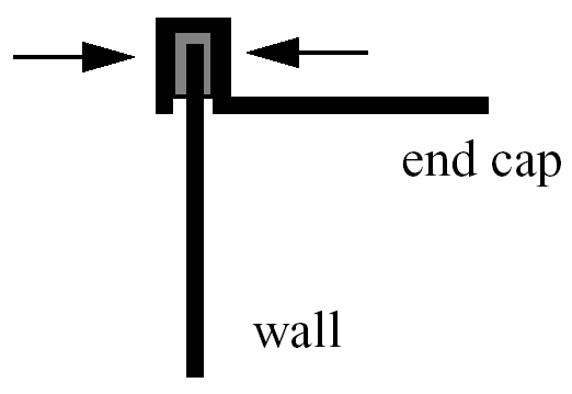
Fig. 17 Container wall-to-end-cap seal

For preliminary design purposes, the extra material that would normally go into the container end cap seals is approximated by increasing the cut dimensions of the end cap diameters by 12% and the height of the container wall by 5%, and waste associated with stamping the end caps in a specialized pattern from sheet stock is estimated as 15% of the cap area. The equation for the area of the container materials including waste is

$$\begin{array}{r}A=2\times \left(\begin{array}{c}\mathtt{end}\mathtt{cap}\\ \mathtt{waste}\\ \mathtt{material}\\ \mathtt{factor}\end{array}\right)\times \left(\begin{array}{c}\mathtt{end}\mathtt{cap}\\ \mathtt{seal}\\ \mathtt{material}\\ \mathtt{factor}\end{array}\right)\times \left(\begin{array}{c}\mathtt{nominal}\\ \mathtt{end}\mathtt{cap}\\ \mathtt{area}\end{array}\right)+\left(\begin{array}{c}\mathtt{container}\\ \mathtt{wall}\mathtt{seal}\\ \mathtt{material}\\ \mathtt{factor}\end{array}\right)\times \left(\begin{array}{c}\mathtt{nominal}\\ \mathtt{container}\\ \mathtt{wall}\mathtt{area}\end{array}\right)\end{array}$$

or

(13)$$A=2(1.15)(1.12)\pi \frac{D^2}{4}+(1.05)\pi DH$$

where $D$ and $H$ are the diameter and height of the finished product in units of inches, respectively. The volume of the finished product is specified to be

(14)$$V=\pi \frac{D^{2}H}{4}=(1.1\mathtt{qt})(57.75{\mathtt{in}}^3/\mathtt{qt})$$

The equation for area is the objective function for this problem; it is to be minimized. The equation for volume is an equality constraint; it must be satisfied at the conclusion of the optimization problem. Any combination of $D$ and $H$ that satisfies the volume constraint is a feasible solution (although not necessarily the optimal solution) to the area minimization problem, and any combination that does not satisfy the volume constraint is an infeasible solution. The area that is a minimum subject to the volume constraint is the optimal area, and the corresponding values for the parameters $D$ and $H$ are the optimal parameter values.

It is important that the equations supplied to a numerical optimization code be limited to generating only physically realizable values, since an optimizer will not have the capability to differentiate between meaningful and nonphysical parameter values. It is often up to the engineer to supply these limits, usually in the form of parameter bound constraints. For example, by observing the equations for the area objective function and the volume constraint, it can be seen that by allowing the diameter, $D$, to become negative, it is algebraically possible to generate relatively small values for the area that also satisfy the volume constraint. Negative values for $D$ are of course physically meaningless. Therefore, to ensure that the numerically-solved optimization problem remains meaningful, a bound constraint of $-D\le 0$ must be included in the optimization problem statement. A positive value for $H$ is implied since the volume constraint could never be satisfied if $H$ were negative. However, a bound constraint of $-H\le 0$ can be added to the optimization problem if desired. The optimization problem can then be stated in a standardized form as

(15)$$\begin{array}{rl}\mathtt{\text{minimize }}& 2(1.15)(1.12)\pi \frac{D^2}{4}+(1.05{)}^2\pi DH\\ \mathtt{\text{subject to }}& \pi \frac{D^{2}H}{4}=(1.1\mathtt{qt})(57.75{\mathtt{in}}^3/\mathtt{qt})\\ & -D\le 0\text{, }-H\le 0\end{array}$$

A graphical view of the container optimization test problem appears in Fig. 18. The 3-D surface defines the area, $A$, as a function of diameter and height. The curved line that extends across the surface defines the areas that satisfy the volume equality constraint, $V$. Graphically, the container optimization problem can be viewed as one of finding the point along the constraint line with the smallest 3-D surface height in Fig. 18. This point corresponds to the optimal values for diameter and height of the final product.

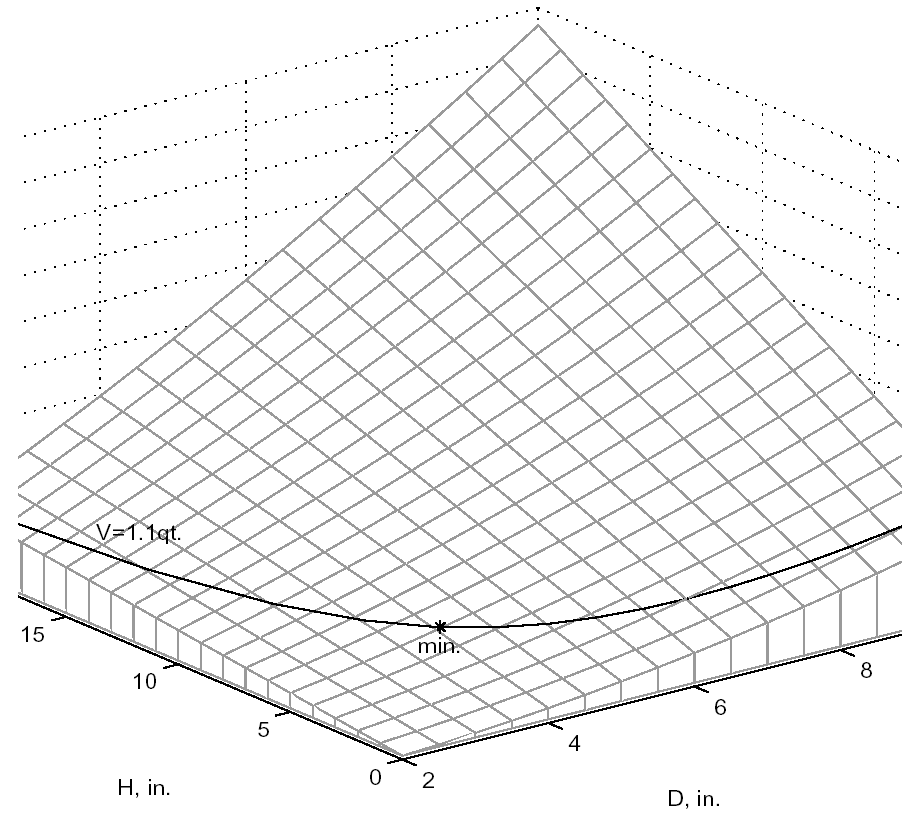
Fig. 18 A graphical representation of the container optimization problem.

Constrained Gradient Based Optimization

The input file for this example is named container_opt_npsol.in. The solution to this example problem is $(H,D)=(4.99,4.03)$, with a minimum area of 98.43 ${\mathtt{in}}^2$ .

The final report from the Dakota output is as follows:

<<<<< Iterator npsol_sqp completed.
<<<<< Function evaluation summary: 40 total (40 new, 0 duplicate)
<<<<< Best parameters          =
                      4.9873894231e+00 H
                      4.0270846274e+00 D
<<<<< Best objective function  =
                      9.8432498116e+01
<<<<< Best constraint values   =
                     -9.6301439045e-12
<<<<< Best evaluation ID: 36
<<<<< Environment execution completed.
Dakota execution time in seconds:
  Total CPU        =      0.18 [parent =      0.18, child =         0]
  Total wall clock =  0.809126

Cantilever

This test problem is adapted from the reliability-based design optimization literature:cite:p:Sue01, [WSSC01] and involves a simple uniform cantilever beam as shown in Fig. 19.

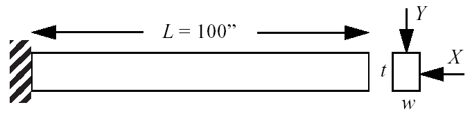
Fig. 19 Cantilever beam test problem.

The design problem is to minimize the weight (or, equivalently, the cross-sectional area) of the beam subject to a displacement constraint and a stress constraint. Random variables in the problem include the yield stress $R$ of the beam material, the Young’s modulus $E$ of the material, and the horizontal and vertical loads, $X$ and $Y$, which are modeled with normal distributions using $N(40000,2000)$, $N(2.9E7,1.45E6)$, $N(500,100)$, and $N(1000,100)$, respectively. Problem constants include $L=100\mathtt{in}$ and $D_0=2.2535\mathtt{in}$. The constraints have the following analytic form:

(16)$$\begin{array}{rl}\mathtt{stress}& =\frac{600}{w{t}^2}Y+\frac{600}{w^{2}t}X\le R\\ \mathtt{displacement}& =\frac{4L^3}{Ewt}\sqrt{(\frac{Y}{t^2}{)}^2+(\frac{X}{w^2}{)}^2}\le D_0\end{array}$$

or when scaled:

(17)$$\begin{array}{rl}{g}_S& =\frac{\mathtt{stress}}{R}-1\le 0\\ g_D& =\frac{\mathtt{displacement}}{D_0}-1\le 0\end{array}$$

Deterministic Formulation: If the random variables $E$, $R$, $X$, and $Y$ are fixed at their means, the resulting deterministic design problem can be formulated as

(18)$$\begin{array}{rl}\mathtt{\text{minimize }}& f=wt\\ \mathtt{\text{subject to }}& g_S\le 0\\ & g_D\le 0\\ & 1.0\le w\le 4.0\\ & 1.0\le t\le 4.0\end{array}$$

Stochastic Formulation: If the normal distributions for the random variables $E$, $R$, $X$, and $Y$ are included, a stochastic design problem can be formulated as

(19)$$\begin{array}{rl}\mathtt{\text{minimize }}& f=wt\\ \mathtt{\text{subject to }}& {\beta }_D\ge 3\\ & {\beta }_S\ge 3\\ & 1.0\le w\le 4.0\\ & 1.0\le t\le 4.0\end{array}$$

where a 3-sigma reliability level (probability of failure = 0.00135 if responses are normally-distributed) is being sought on the scaled constraints.

Constrained Gradient Based Optimization

Here, the Cantilever test problem is solved using cantilever_opt_npsol.in:

Listing 8 Cantilever Example: the Dakota input file – see dakota/share/dakota/examples/users/cantilever_opt_npsol.in

# Dakota Input File: cantilever_opt_npsol.in

method
# (NPSOL requires a software license; if not available, try
# conmin_mfd or optpp_q_newton instead)
  npsol_sqp
    convergence_tolerance = 1.e-8

variables
  continuous_design = 2
    initial_point  4.0   4.0
    upper_bounds  10.0  10.0
    lower_bounds   1.0   1.0
    descriptors    'w'   't'
  continuous_state = 4
    initial_state  40000. 29.E+6 500. 1000.
    descriptors      'R'   'E'   'X'   'Y'

interface
  analysis_drivers = 'cantilever'
    fork
  asynchronous evaluation_concurrency = 2

responses
  objective_functions = 1
  nonlinear_inequality_constraints = 2
  numerical_gradients
    method_source dakota
    interval_type forward
    fd_step_size = 1.e-4
  no_hessians

The deterministic solution is $(w,t)=(2.35,3.33)$ with an objective function of $7.82$. The final report from the Dakota output is as follows:

<<<<< Iterator npsol_sqp completed.
<<<<< Function evaluation summary: 33 total (33 new, 0 duplicate)
<<<<< Best parameters          =
                      2.3520341271e+00 beam_width
                      3.3262784077e+00 beam_thickness
                      4.0000000000e+04 R
                      2.9000000000e+07 E
                      5.0000000000e+02 X
                      1.0000000000e+03 Y
<<<<< Best objective function  =
                      7.8235203313e+00
<<<<< Best constraint values   =
                     -1.6009000260e-02
                     -3.7083558446e-11
<<<<< Best evaluation ID: 31
<<<<< Environment execution completed.
Dakota execution time in seconds:
  Total CPU        =       0.03 [parent =   0.027995, child =   0.002005]
  Total wall clock =   0.281375

Optimization Under Uncertainty

Optimization under uncertainty solutions to the stochastic problem are described in [EAP+07, EB06, EGWojtkiewiczJrT02], for which the solution is $(w,t)=(2.45,3.88)$ with an objective function of $9.52$. This demonstrates that a more conservative design is needed to satisfy the probabilistic constraints.

Multiobjective Test Problems

Multiobjective optimization means that there are two or more objective functions that you wish to optimize simultaneously. Often these are conflicting objectives, such as cost and performance. The answer to a multi-objective problem is usually not a single point. Rather, it is a set of points called the Pareto front. Each point on the Pareto front satisfies the Pareto optimality criterion, i.e., locally there exists no other feasible vector that would improve some objective without causing a simultaneous worsening in at least one other objective. Thus a feasible point $X^{\prime }$ from which small moves improve one or more objectives without worsening any others is not Pareto optimal: it is said to be “dominated” and the points along the Pareto front are said to be “non-dominated”.

Often multi-objective problems are addressed by simply assigning weights to the individual objectives, summing the weighted objectives, and turning the problem into a single-objective one which can be solved with a variety of optimization techniques. While this approach provides a useful “first cut” analysis (and is supported within Dakota – see Multiobjective Optimization), this approach has many limitations. The major limitation is that a local solver with a weighted sum objective will only find one point on the Pareto front; if one wants to understand the effects of changing weights, this method can be computationally expensive. Since each optimization of a single weighted objective will find only one point on the Pareto front, many optimizations must be performed to get a good parametric understanding of the influence of the weights and to achieve a good sampling of the entire Pareto frontier.

There are three examples that are taken from a multiobjective evolutionary algorithm (MOEA) test suite described by Van Veldhuizen et. al. in [CVVL02]. These three examples illustrate the different forms that the Pareto set may take. For each problem, we describe the Dakota input and show a graph of the Pareto front. These problems are all solved with the moga method. The first example is discussed in Multiobjective Optimization, which also provides more information on multiobjective optimization. The other two are described below.

Multiobjective Test Problem 2

The second test problem is a case where both ${\mathtt{P}}_{\mathtt{true}}$ and ${\mathtt{PF}}_{\mathtt{true}}$ are disconnected. ${\mathtt{PF}}_{\mathtt{true}}$ has four separate Pareto curves. The problem is to simultaneously optimize $f_1$ and $f_2$ given two input variables, $x_1$ and $x_2$, where the inputs are bounded by $0\le x_i\le 1$, and:

$$\begin{array}{rl}{f}_1(x)& =x_1\\ f_2(x)& =(1+10x_2)\times [1-(\frac{x_1}{1+10x_2}{)}^2-\frac{x_1}{1+10x_2}\sin (8\pi x_1)]\end{array}$$

The input file for this example is shown in Listing 9, which references the mogatest2 executable (compiled from dakota_source/test/mogatest2.cpp) as the simulator. The Pareto front is shown in Fig. 20. Note the discontinuous nature of the front in this example.

Listing 9 Dakota input file specifying the use of MOGA on mogatest2 – see dakota/share/dakota/examples/users/mogatest2.in

# Dakota Input File: mogatest2.in

environment
  tabular_data
    tabular_data_file = 'mogatest2.dat'

method
  moga
    seed = 10983
  max_function_evaluations = 3000
  initialization_type unique_random
  crossover_type
    multi_point_parameterized_binary = 2
    crossover_rate = 0.8
  mutation_type replace_uniform
    mutation_rate = 0.1
  fitness_type domination_count
  replacement_type below_limit = 6
    shrinkage_fraction = 0.9
  convergence_type metric_tracker
    percent_change = 0.05 num_generations = 10
  final_solutions = 3
  output silent

variables
  continuous_design = 2
    initial_point    0.5      0.5
    upper_bounds     1         1
    lower_bounds     0         0
    descriptors      'x1'   'x2'

interface
  analysis_drivers = 'mogatest2'
    direct

responses
  objective_functions = 2
  no_gradients
  no_hessians

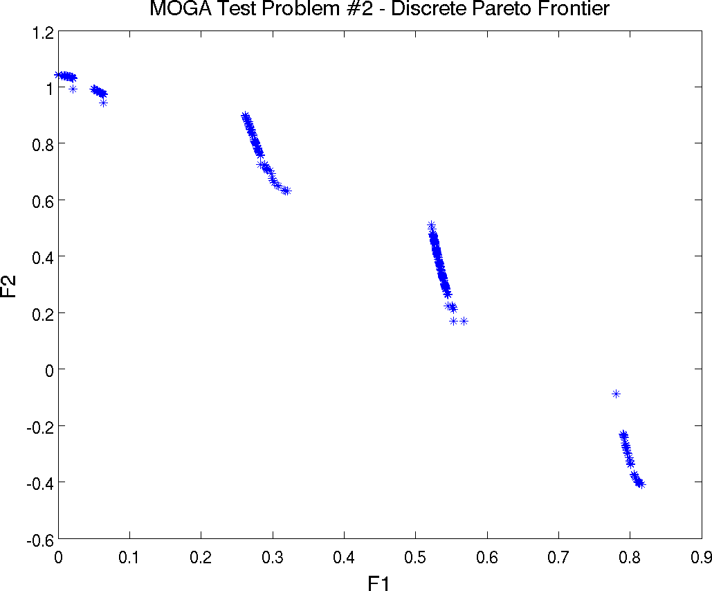
Fig. 20 Pareto Front showing Tradeoffs between Function F1 and Function F2 for mogatest2

Multiobjective Test Problem 3

The third test problem is a case where ${\mathtt{P}}_{\mathtt{true}}$ is disconnected but ${\mathtt{PF}}_{\mathtt{true}}$ is connected. This problem also has two nonlinear constraints. The problem is to simultaneously optimize $f_1$ and $f_2$ given two input variables, $x_1$ and $x_2$, where the inputs are bounded by $-20\le x_i\le 20$, and:

$$\begin{array}{rl}{f}_1(x)& =(x_1-2{)}^2+(x_2-1{)}^2+2\\ f_2(x)& =9x_1-(x_2-1{)}^2\end{array}$$

The constraints are:

$$\begin{array}{rl}0& \le x_1^2+x_2^2-225\\ 0& \le x_1-3x_2+10\end{array}$$

The input file for this example is shown in Listing 10. It differs from Listing 9 in the variables and responses specifications, in the use of the mogatest3 executable (compiled from dakota_source/test/mogatest3.cpp) as the simulator, and in the max_function_evaluations and mutation_type MOGA controls. The Pareto set is shown in Fig. 21. Note the discontinuous nature of the Pareto set (in the design space) in this example. The Pareto front is shown in Fig. 22.

Listing 10 Dakota input file specifying the use of MOGA on mogatest3 – see dakota/share/dakota/examples/users/mogatest3.in

# Dakota Input File: mogatest3.in

environment
  tabular_data
    tabular_data_file = 'mogatest3.dat'

method
  moga
    seed = 10983
  max_function_evaluations = 2000
  initialization_type unique_random
  crossover_type
    multi_point_parameterized_binary = 2
    crossover_rate = 0.8
  mutation_type offset_normal
    mutation_scale = 0.1
  fitness_type domination_count
  replacement_type below_limit = 6
    shrinkage_fraction = 0.9
  convergence_type metric_tracker
    percent_change = 0.05 num_generations = 10
  final_solutions = 3
  output silent

variables
  continuous_design = 2
    descriptors      'x1'   'x2'
    initial_point      0     0
    upper_bounds      20    20
    lower_bounds     -20   -20

interface
  analysis_drivers = 'mogatest3'
    direct

responses
  objective_functions = 2
  nonlinear_inequality_constraints = 2
    upper_bounds = 0.0 0.0
  no_gradients
  no_hessians

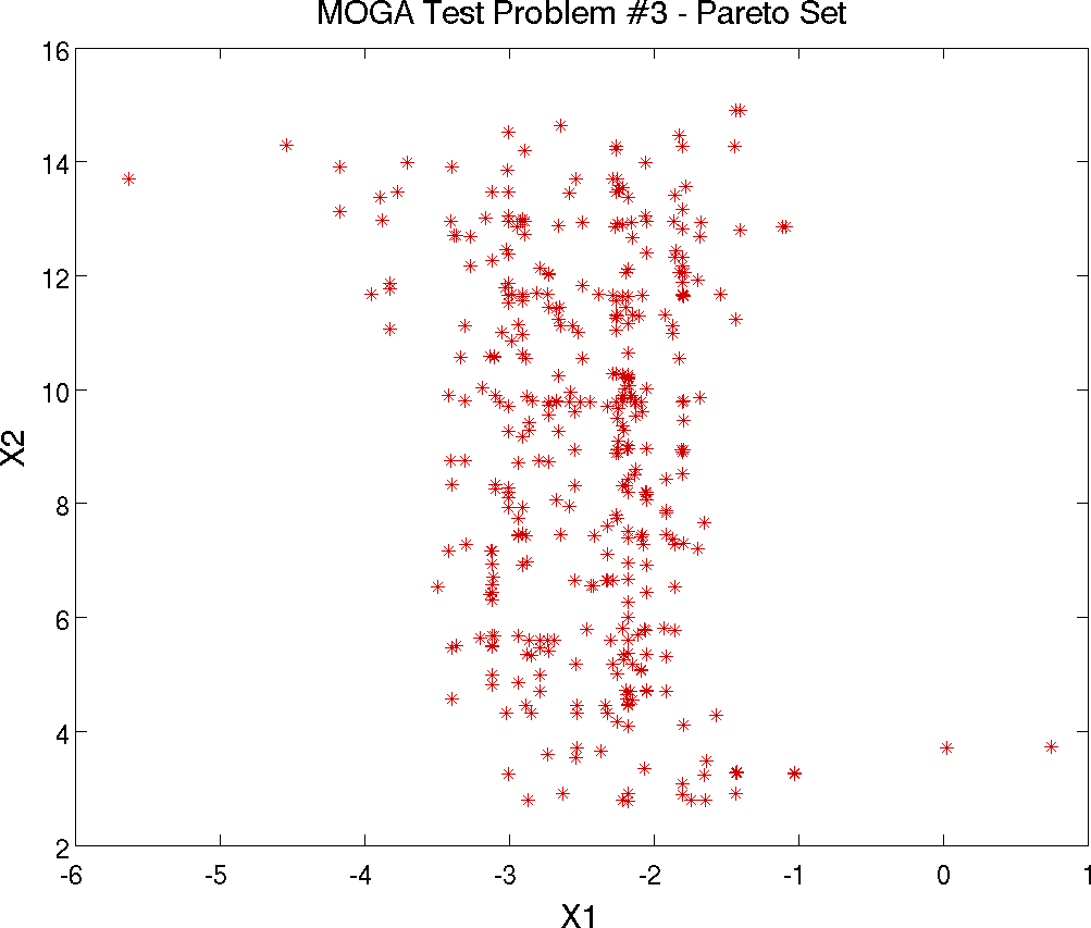
Fig. 21 Pareto Set of Design Variables corresponding to the Pareto front for mogatest3

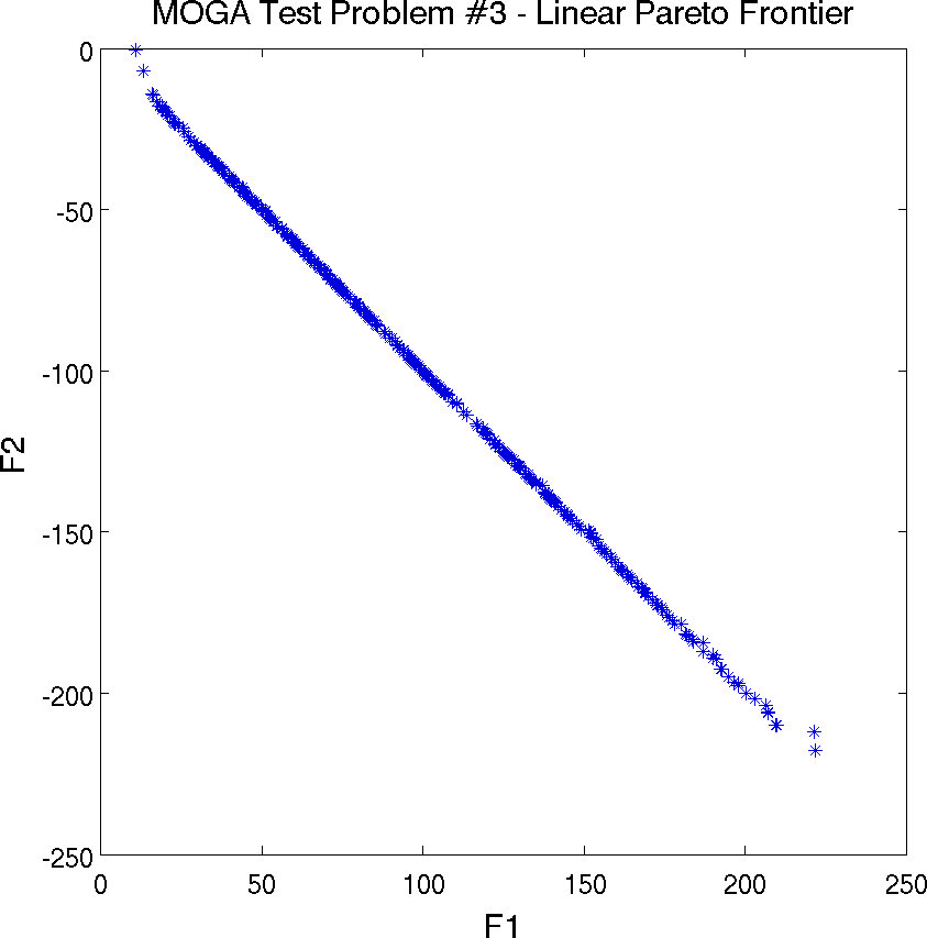
Fig. 22 Pareto Front showing Tradeoffs between Function F1 and Function F2 for mogatest3

Morris

Morris [Mor91] includes a screening design test problem with a single-output analytical test function. The output depends on 20 inputs with first- through fourth-order interaction terms, some having large fixed coefficients and others small random coefficients. Thus the function values generated depend on the random number generator employed in the function evaluator. The computational model is:

$$\begin{array}{rl}y=& {\beta }_0+\sum _{i=1}^{20}{\beta }_i{w}_i+\sum _{i<j}^{20}{\beta }_{i,j}{w}_i{w}_j+\sum _{i<j<l}^{20}{\beta }_{i,j,l}{w}_i{w}_j{w}_l\\ & +\sum _{i<j<l<s}^{20}{\beta }_{i,j,l,s}{w}_i{w}_j{w}_l{w}_s,\end{array}$$

where $w_i=2(x_i-0.5)$ except for $i=3,5,\text{ and }7$, where $w_i=2(1.1x_i/(x_i+0.1)-0.5)$. Large-valued coefficients are assigned as

$$\begin{array}{rlrlrl}{\beta }_i=+20& & i=1,\dots ,10;& {\beta }_{i,j}=-15& & i,j=1,\dots ,6;\\ {\beta }_{i,j,l}=-10& & i,j,l=1,\dots ,5;& {\beta }_{i,j,l,s}=+5& & i,j,l,s=1,\dots ,4.\end{array}$$

The remaining first- and second-order coefficients ${\beta }_i$ and ${\beta }_{i,j}$, respectively, are independently generated from a standard normal distribution (zero mean and unit standard deviation); the remaining third- and fourth-order coefficients are set to zero.

Examination of the test function reveals that one should be able to conclude the following (stated and verified computationally in [STCR04]) for this test problem:

1. the first ten factors are important;

2. of these, the first seven have significant effects involving either interactions or curvatures; and

3. the other three are important mainly because of their first-order effect.

Morris One-at-a-Time Sensitivity Study

The dakota input morris_ps_moat.in exercises the MOAT algorithm described in PSUADE MOAT on the Morris problem. The Dakota output obtained is shown in Listing 11 and Listing 12.

Listing 11 Dakota MOAT output: preamble.

Running MPI executable in serial mode.
Dakota version 6.0 release.
Subversion revision xxxx built May ...
Writing new restart file dakota.rst
gradientType = none
hessianType = none

>>>>> Executing environment.

>>>>> Running psuade_moat iterator.

PSUADE DACE method = psuade_moat Samples = 84 Seed (user-specified) = 500
            Partitions = 3 (Levels = 4)

Listing 12 Dakota MOAT output: final results.

>>>>>> PSUADE MOAT output for function 0:

*************************************************************
*********************** MOAT Analysis ***********************
-------------------------------------------------------------
Input   1 (mod. mean & std) =   9.5329e+01   9.0823e+01
Input   2 (mod. mean & std) =   6.7297e+01   9.5242e+01
Input   3 (mod. mean & std) =   1.0648e+02   1.5479e+02
Input   4 (mod. mean & std) =   6.6231e+01   7.5895e+01
Input   5 (mod. mean & std) =   9.5717e+01   1.2733e+02
Input   6 (mod. mean & std) =   8.0394e+01   9.9959e+01
Input   7 (mod. mean & std) =   3.2722e+01   2.7947e+01
Input   8 (mod. mean & std) =   4.2013e+01   7.6090e+00
Input   9 (mod. mean & std) =   4.1965e+01   7.8535e+00
Input  10 (mod. mean & std) =   3.6809e+01   3.6151e+00
Input  11 (mod. mean & std) =   8.2655e+00   1.0311e+01
Input  12 (mod. mean & std) =   4.9299e+00   7.0591e+00
Input  13 (mod. mean & std) =   3.5455e+00   4.4025e+00
Input  14 (mod. mean & std) =   3.4151e+00   2.4905e+00
Input  15 (mod. mean & std) =   2.5143e+00   5.5168e-01
Input  16 (mod. mean & std) =   9.0344e+00   1.0115e+01
Input  17 (mod. mean & std) =   6.4357e+00   8.3820e+00
Input  18 (mod. mean & std) =   9.1886e+00   2.5373e+00
Input  19 (mod. mean & std) =   2.4105e+00   3.1102e+00
Input  20 (mod. mean & std) =   5.8234e+00   7.2403e+00
<<<<< Function evaluation summary: 84 total (84 new, 0 duplicate)

The MOAT analysis output reveals that each of the desired observations can be made for the test problem. These are also reflected in Fig. 23. The modified mean (based on averaging absolute values of elementary effects) shows a clear difference in inputs 1–10 as compared to inputs 11–20. The standard deviation of the (signed) elementary effects indicates correctly that inputs 1–7 have substantial interaction-based or nonlinear effect on the output, while the others have less. While some of inputs 11–20 have nontrivial values of $\sigma$, their relatively small modified means ${\mu }^{\ast }$ indicate they have little overall influence.

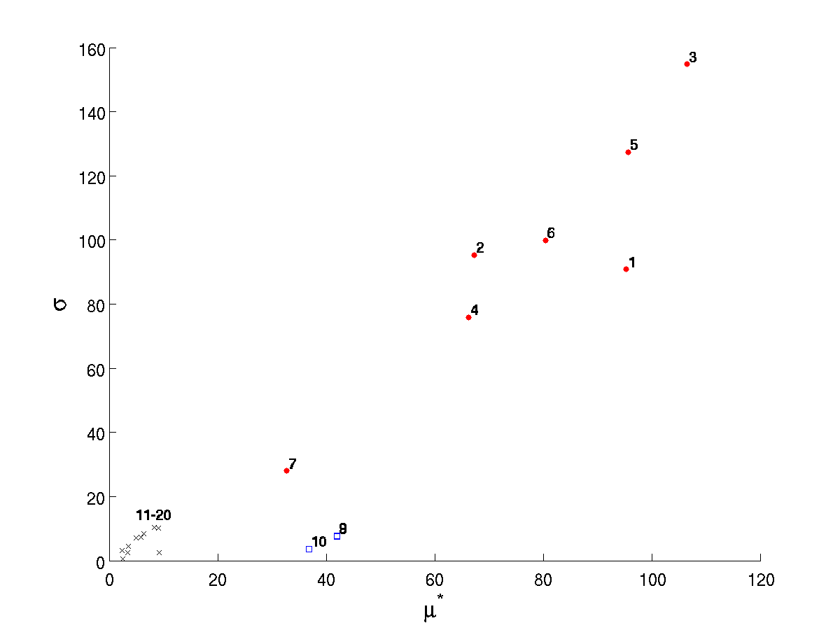
Fig. 23 Standard deviation of elementary effects plotted against modified mean for Morris for each of 20 inputs. Red circles 1–7 correspond to inputs having interactions or nonlinear effects, blue squares 8–10 indicate those with mainly linear effects, and black Xs denote insignificant inputs.

Test Problems for Reliability Analyses

This section includes several test problems and examples related to reliability analyses.

Note

These are included in the dakota/share/dakota/examples/users directory, rather are in the dakota/share/dakota/test directory.

Log Ratio

This test problem, mentioned previously in Uncertainty Quantification Examples using Reliability Analysis, has a limit state function defined by the ratio of two lognormally-distributed random variables.

$$g(\mathbf{x})=\frac{x_1}{x_2}$$

The distributions for both $x_1$ and $x_2$ are Lognormal(1, 0.5) with a correlation coefficient between the two variables of 0.3.

Reliability Analyses

First-order and second-order reliability analysis (FORM and SORM) are performed in dakota/share/dakota/examples/users/logratio_uq_reliability.in and dakota/share/dakota/test/dakota_logratio_taylor2.in.

For the reliability index approach (RIA), 24 response levels (.4, .5, .55, .6, .65, .7, .75, .8, .85, .9, 1, 1.05, 1.15, 1.2, 1.25, 1.3, 1.35, 1.4, 1.5, 1.55, 1.6, 1.65, 1.7, and 1.75) are mapped into the corresponding cumulative probability levels. For performance measure approach (PMA), these 24 probability levels (the fully converged results from RIA FORM) are mapped back into the original response levels. Fig. 24 and Fig. 25 overlay the computed CDF values for a number of first-order reliability method variants as well as a Latin Hypercube reference solution of ${10}^6$ samples.

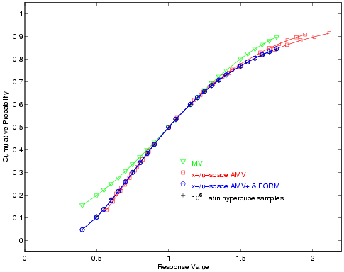
Fig. 24 Lognormal ratio cumulative distribution function, RIA method.

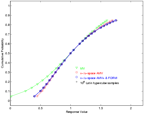
Fig. 25 Lognormal ratio cumulative distribution function, PMA method.

Steel Section

This test problem is used extensively in [HM00]. It involves a W16x31 steel block of A36 steel that must carry an applied deterministic bending moment of 1140 kip-in. For Dakota, it has been used as a code verification test for second-order integrations in reliability methods. The limit state function is defined as:

$$g(\mathbf{x})=F_{y}Z-1140$$

where $F_y$ is Lognormal(38., 3.8), $Z$ is Normal(54., 2.7), and the variables are uncorrelated.

The dakota/share/dakota/test/dakota_steel_section.in input file computes a first-order CDF probability of $p(g\le 0.)=1.297e-07$ and a second-order CDF probability of $p(g\le 0.)=1.375e-07$. This second-order result differs from that reported in [HM00], since Dakota uses the Nataf nonlinear transformation to u-space (see MPP Search Methods for the formulation, while [HM00] uses a linearized transformation.

Portal Frame

This test problem is taken from [Hon99, Tve90]. It involves a plastic collapse mechanism of a simple portal frame. It also has been used as a verification test for second-order integrations in reliability methods. The limit state function is defined as:

$$g(\mathbf{x})=x_1+2x_2+2x_3+x_4-5x_5-5x_6$$

where $x_1-x_4$ are Lognormal(120., 12.), $x_5$ is Lognormal(50., 15.), $x_6$ is Lognormal(40., 12.), and the variables are uncorrelated.

While the limit state is linear in x-space, the nonlinear transformation of lognormals to u-space induces curvature. The input file dakota/share/dakota/test/dakota_portal_frame.in computes a first-order CDF probability of $p(g\le 0.)=9.433e-03$ and a second-order CDF probability of $p(g\le 0.)=1.201e-02$. These results agree with the published results from the literature.

Short Column

This test problem involves the plastic analysis and design of a short column with rectangular cross section (width $b$ and depth $h$) having uncertain material properties (yield stress $Y$) and subject to uncertain loads (bending moment $M$ and axial force $P$) [KR97]. The limit state function is defined as:

$$g(\mathbf{x})=1-\frac{4M}{b{h}^{2}Y}-\frac{P^2}{b^2{h}^2{Y}^2}$$

The distributions for $P$, $M$, and $Y$ are Normal(500, 100), Normal(2000, 400), and Lognormal(5, 0.5), respectively, with a correlation coefficient of 0.5 between $P$ and $M$ (uncorrelated otherwise). The nominal values for $b$ and $h$ are 5 and 15, respectively.

Reliability Analyses

First-order and second-order reliability analysis are performed in the dakota_short_column.in and dakota_short_column_taylor2.in input files in dakota/share/dakota/test. For RIA, 43 response levels (-9.0, -8.75, -8.5, -8.0, -7.75, -7.5, -7.25, -7.0, -6.5, -6.0, -5.5, -5.0, -4.5, -4.0, -3.5, -3.0, -2.5, -2.0, -1.9, -1.8, -1.7, -1.6, -1.5, -1.4, -1.3, -1.2, -1.1, -1.0, -0.9, -0.8, -0.7, -0.6, -0.5, -0.4, -0.3, -0.2, -0.1, 0.0, 0.05, 0.1, 0.15, 0.2, 0.25) are mapped into the corresponding cumulative probability levels. For PMA, these 43 probability levels (the fully converged results from RIA FORM) are mapped back into the original response levels. Fig. 26 and Fig. 27 overlay the computed CDF values for several first-order reliability method variants as well as a Latin Hypercube reference solution of ${10}^6$ samples.

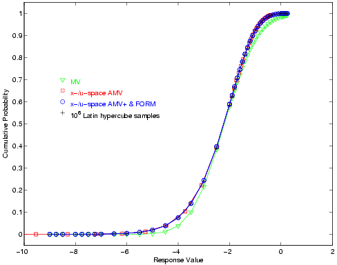
Fig. 26 Short column cumulative distribution function, RIA method.

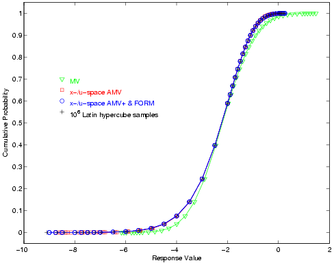
Fig. 27 Short column cumulative distribution function, PMA method.

Reliability-Based Design Optimization

The short column test problem is also amenable to Reliability-Based Design Optimization (RBDO). An objective function of cross-sectional area and a target reliability index of 2.5 (cumulative failure probability $p(g\le 0)\le 0.00621$) are used in the design problem:

$$\begin{array}{rl}min& bh\\ \text{s.t.}& \beta \ge 2.5\\ & 5.0\le b\le 15.0\\ & 15.0\le h\le 25.0\end{array}$$

As is evident from the UQ results shown in Fig. 26 or Fig. 27, the initial design of $(b,h)=(5,15)$ is infeasible and the optimization must add material to obtain the target reliability at the optimal design $(b,h)=(8.68,25.0)$. Simple bi-level, fully analytic bi-level, and sequential RBDO methods are explored in input files dakota_rbdo_short_column.in, dakota_rbdo_short_column_analytic.in, and dakota_rbdo_short_column_trsb.in, with results as described in [EAP+07, EB06]. These files are located in dakota/share/dakota/test.

Steel Column

This test problem involves the trade-off between cost and reliability for a steel column [KR97]. The cost is defined as

$$Cost=bd+5h$$

where $b$, $d$, and $h$ are the means of the flange breadth, flange thickness, and profile height, respectively. Nine uncorrelated random variables are used in the problem to define the yield stress $F_s$ (lognormal with $\mu /\sigma$ = 400/35 MPa), dead weight load $P_1$ (normal with $\mu /\sigma$ = 500000/50000 N), variable load $P_2$ (gumbel with $\mu /\sigma$ = 600000/90000 N), variable load $P_3$ (gumbel with $\mu /\sigma$ = 600000/90000 N), flange breadth $B$ (lognormal with $\mu /\sigma$ = $b$/3 mm), flange thickness $D$ (lognormal with $\mu /\sigma$ = $d$/2 mm), profile height $H$ (lognormal with $\mu /\sigma$ = $h$/5 mm), initial deflection $F_0$ (normal with $\mu /\sigma$ = 30/10 mm), and Young’s modulus $E$ (Weibull with $\mu /\sigma$ = 21000/4200 MPa). The limit state has the following analytic form:

$$g=F_s-P(\frac{1}{2BD}+\frac{F_0}{BDH}\frac{E_b}{E_b-P})$$

where

$$\begin{array}{rl}P& =P_1+P_2+P_3\\ E_b& =\frac{{\pi }^{2}EBD{H}^2}{2L^2}\end{array}$$

and the column length $L$ is 7500 mm.

This design problem (dakota_rbdo_steel_column.in in dakota/share/dakota/test) demonstrates design variable insertion into random variable distribution parameters through the design of the mean flange breadth, flange thickness, and profile height. The RBDO formulation maximizes the reliability subject to a cost constraint:

$$\begin{array}{rl}\text{maximize }& \beta \\ \text{subject to }& Cost\le 4000.\\ & 200.0\le b\le 400.0\\ & 10.0\le d\le 30.0\\ & 100.0\le h\le 500.0\end{array}$$

which has the solution $(b,d,h)=(200.0,17.50,100.0)$ with a maximal reliability of 3.132.

Test Problems for Forward UQ

This section includes several test problems and examples related to forward uncertainty quantification.

Note

These are not included in the dakota/share/dakota/examples/users directory, rather are in the dakota/share/dakota/test directory.

Genz functions

The Genz functions have traditionally been used to test quadrature methods, however more recently they have also been used to test forward UQ methdos. Here we consider the oscilatory and corner-peak test functions, respectively given by

$$f_{\mathrm{OS}}(\mathit{\xi })=\cos (-\sum _{i=1}^d{c}_i{\xi }_i),\mathit{\xi }\in [0,1{]}^d$$

$$f_{\mathrm{CP}}(\mathit{\xi })={(1+\sum _{i=1}^d{c}_i{\xi }_i)}^{-(d+1)},\mathit{\xi }\in [0,1{]}^d$$

The coefficients $c_k$ can be used to control the effective dimensionality and the variability of these functions. In dakota we support three choices of $\mathbf{=}(c_1,\dots ,c_d{)}^T$, specifically

$$c_k^{(1)}=\frac{k-\frac{1}{2}}{d},c_k^{(2)}=\frac{1}{k^2}\text{and}{c}_k^{(3)}=\exp \left(\frac{k\log ({10}^{-8})}{d}\right),k=1,\dots ,d$$

normalizing such that for the oscillatory function $\sum _{k=1}^d{c}_k=4.5$ and for the corner peak function $\sum _{k=1}^d{c}_k=0.25$. The different decay rates of the coefficients represent increasing levels of anisotropy and decreasing effective dimensionality. Anisotropy refers to the dependence of the function variability.

In Dakota the genz function can be set by specifying analysis_driver=’genz’. The type of coefficients decay can be set by specifying os1, cp1 which uses ${\mathbf{c}}^{(1)}$, os2, cp2 which uses ${\mathbf{c}}^{(2)}$, and os3, cp3 which uses ${\mathbf{c}}^{(3)}$, where os is to be used with the oscillatory function and cp for the corner peak function.

Elliptic Partial differential equation with uncertain coefficients

Consider the following problem with $d\ge 1$ random dimensions:

(20)$$-\frac{d}{dx}[a(x,\mathit{\xi })\frac{du}{dx}(x,\mathit{\xi })]=10,(x,\mathit{\xi })\in (0,1)\times I_{\mathit{\xi }}$$

subject to the physical boundary conditions

$$u(0,\mathit{\xi })=0,u(1,\mathit{\xi })=0.$$

We are interested in quantifying the uncertainty in the solution $u$ at a number of locations $x\in [0,1]$ which can be specified by the user. This function can be run using dakota by specifying analysis_driver='steady_state_diffusion_1d'.

We represent the random diffusivity field $a$ using two types of expansions. The first option is to use represent the logarithm of the diffusivity field as Karhunen Loéve expansion

(21)$$\log (a(x,\mathit{\xi }))=\overline{a}+{\sigma }_a\sum _{k=1}^d\sqrt{{\lambda }_k}{\varphi }_k(x){\xi }_k$$

where $\{{\lambda }_k{\}}_{k=1}^d$ and $\{{\varphi }_k(x){\}}_{k=1}^d$ are, respectively, the eigenvalues and eigenfunctions of the covariance kernel

(22)$$C_a(x_1,x_2)=\exp [-\frac{(x_1-x_2{)}^p}{l_c}].$$

for some power $p=1,2$. The variability of the diffusivity field (21) is controlled by ${\sigma }_a$ and the correlation length $l_c$ which determines the decay of the eigenvalues ${\lambda }_k$. Dakota sets ${\sigma }_a=1.$ but allows the number of random variables $d$, the order of the kernel $p$ and the correlation length $l_c$ to vary. The random variables can be bounded or unbounded.

The second expansion option is to represent the diffusivity by

(23)$$a(x,\mathit{\xi })=1+\sigma \sum _{k=1}^d\frac{1}{k^2{\pi }^2}\cos (2\pi kx){\mathit{\xi }}_k$$

where ${\mathit{\xi }}_k\in [-1,1]$, $k=1,\dots ,d$ are bounded random variables. The form of (23) is similar to that obtained from a Karhunen-Loève expansion. If the variables are i.i.d. uniform in [-1,1] the the diffusivity satisfies satisfies the auxiliary properties

$$\mathbb{E}[a(x,\mathit{\xi })]=1\text{and}1-\frac{\sigma }{6}<a(x,\mathit{\xi })<1+\frac{\sigma }{6}.$$

This is the same test case used in [XH05].

Damped Oscillator

Consider a damped linear oscillator subject to external forcing with six unknown parameters $\mathit{\xi }=(\gamma ,k,f,\omega ,x_0,x_1)$

(24)$$\frac{d^{2}x}{d{t}^2}(t,\mathit{\xi })+\gamma \frac{dx}{dt}+kx=f\cos (\omega t),$$

subject to the initial conditions

$$x(0)=x_0,\dot{x}(0)=x_1.$$

Here we assume the damping coefficient $\gamma$, spring constant $k$, forcing amplitude $f$ and frequency $\omega$, and the initial conditions $x_0$ and $x_1$ are all uncertain.

This test function can be specified with analysis_driver='damped_oscillator'. This function only works with the uncertain variables defined over certain ranges. These ranges are

$${\gamma }_k\in [0.08,0.12],k\in [0.03,0.04],f\in [0.08,0.12],\omega \in [0.8,1.2],x_0\in [0.45,0.55],x_1\in [-0.05,0.05].$$

Do not use this function with unbounded variables, however any bounded variables such as Beta and trucated Normal variables that satisfy the aforementioned variable bounds are fine.

Non-linear coupled system of ODEs

Consider the non-linear system of ordinary differential equations governing a competitive Lotka–Volterra model of the population dynamics of species competing for some common resource. The model is given by

(25)$$\begin{array}{r}\{\begin{array}{ll}\frac{d{u}_i}{dt}=r_i{u}_i(1-\sum _{j=1}^3{\alpha }_{ij}{u}_j),& t\in (0,10],\\ u_i(0)=u_{i,0},\end{array}\end{array}$$

for $i=1,2,3$. The initial condition, $u_{i,0}$, and the self-interacting terms, ${\alpha }_{ii}$, are given, but the remaining interaction parameters, ${\alpha }_{ij}$ with $i\ne j$ as well as the re-productivity parameters, $r_i$, are unknown. We approximate the solution to (25) in time using a Backward Euler method. This test function can be specified with analysis_driver='predator_prey'.

We assume that these parameters are bounded. We have tested this model with all 9 parameters ${\xi }_i\in [0.3,0.7]$. However larger bounds are probably valid. When using the aforemetioned ranges and $1000$ time steps with $\mathrm{\Delta }t=0.01$ the average (over the random parameters) deterministic error is approximately $1.00\times {10}^{-4}$.

Dakota returns the population of each species $u_i(T)$ at the final time $T$. The final time and the number of time-steps can be changed.

Test Problems for Inverse UQ

Experimental Design

This example tests the Bayesian experimental design algorithm described in Bayesian Experimental Design, in which a low-fidelity model is calibrated to optimally-selected data points of a high-fidelity model. The analysis_driver for the the low and high-fidelity models implement the steady state heat example given in [LSWF16]. The high-fidelity model is the analytic solution to the example described therein,

$$T(x)=c_1\exp (-\gamma x)+c_2\exp (\gamma x)+T_{amb},$$

where

$$\begin{array}{rl}{c}_1& =-\frac{\mathrm{\Phi }}{K\gamma }\left[\frac{\exp (\gamma L)(h+K\gamma )}{\exp (-\gamma L)(h-K\gamma )+\exp (\gamma L)(h+K\gamma )}\right],\\ c_2& =\frac{\mathrm{\Phi }}{K\gamma }+c_1,\\ \gamma & =\sqrt{\frac{2(a+b)h}{abK}}.\end{array}$$

The ambient room temperature $T_{amb}$, thermal conductivity coefficient $K$, convective heat transfer coefficient $h$, source heat flux $\mathrm{\Phi }$, and system dimenions $a$, $b$, and $L$ are all set to constant values. The experimental design variable $x\in [10,70]$, is called a configuration variable in Dakota and is the only variable that also appears in the low-fidelity model,

$$y=A{x}^2+Bx+C.$$

The goal of this example is to calibrate the low-fidelity model parameters $A,B$, and $C$ with the Bayesian experimental design algorithm. Refer to Bayesian Experimental Design for further details regarding the Dakota implementation of this example.

Bayes linear

This is a simple model that is only available by using the direct interface with ’bayes_linear’. The model is discussed extensively in [AHL+14] both on pages 93–102 and in Appendix A. The model is simply the sum of the d input parameters:

$$y=\sum _{i=1}^d{x}_i$$

where the input varaibles $x_i$ can be any uncertain variable type but are typically considered as uniform or normal uncertain inputs.