Reliability Methods

Reliability methods provide an alternative approach to uncertainty quantification which can be less computationally demanding than sampling techniques. Reliability methods for uncertainty quantification are based on probabilistic approaches that compute approximate response function distribution statistics based on specified uncertain variable distributions. These response statistics include response mean, response standard deviation, and cumulative or complementary cumulative distribution functions (CDF/CCDF). These methods are often more efficient at computing statistics in the tails of the response distributions (events with low probability) than sampling based approaches since the number of samples required to resolve a low probability can be prohibitive.

The methods all answer the fundamental question: “Given a set of uncertain input variables, \(\mathbf{X}\) , and a scalar response function, \(g\) , what is the probability that the response function is below or above a certain level, \(\bar{z}\) ?” The former can be written as \(P[g(\mathbf{X}) \le \bar{z}] = \mathit{F}_{g}(\bar{z})\) where \(\mathit{F}_{g}(\bar{z})\) is the cumulative distribution function (CDF) of the uncertain response \(g(\mathbf{X})\) over a set of response levels. The latter can be written as \(P[g(\mathbf{X}) > \bar{z}]\) and defines the complementary cumulative distribution function (CCDF).

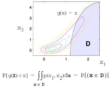
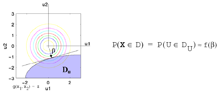
This probability calculation involves a multi-dimensional integral over an irregularly shaped domain of interest, \(\mathbf{D}\) , where \(g(\mathbf{X}) < z\) as displayed in Figure Graphical depiction of calculation of cumulative distribution function in the original uncertain variable space. for the case of two variables. The reliability methods all involve the transformation of the user-specified uncertain variables, \(\mathbf{X}\) , with probability density function, \(p(x_1,x_2)\) , which can be non-normal and correlated, to a space of independent Gaussian random variables, \(\mathbf{u}\) , possessing a mean value of zero and unit variance (i.e., standard normal variables). The region of interest, \(\mathbf{D}\) , is also mapped to the transformed space to yield, \(\mathbf{D_{u}}\) , where \(g(\mathbf{U}) < z\) as shown in Figure Graphical depiction of integration for the calculation of cumulative distribution function in the transformed uncertain variable space.. The Nataf transformation [DKL86], which is identical to the Rosenblatt transformation [Ros52] in the case of independent random variables, is used in Dakota to accomplish this mapping. This transformation is performed to make the probability calculation more tractable. In the transformed space, probability contours are circular in nature as shown in Figure Graphical depiction of integration for the calculation of cumulative distribution function in the transformed uncertain variable space. unlike in the original uncertain variable space, Figure Graphical depiction of calculation of cumulative distribution function in the original uncertain variable space. . Also, the multi-dimensional integrals can be approximated by simple functions of a single parameter, \(\beta\) , called the reliability index. \(\beta\) is the minimum Euclidean distance from the origin in the transformed space to the response surface. This point is also known as the most probable point (MPP) of failure. Note, however, the methodology is equally applicable for generic functions, not simply those corresponding to failure criteria; this nomenclature is due to the origin of these methods within the disciplines of structural safety and reliability. Note that there are local and global reliability methods. The majority of the methods available are local, meaning that a local optimization formulation is used to locate one MPP. In contrast, global methods can find multiple MPPs if they exist.

Fig. 51 Graphical depiction of calculation of cumulative distribution function in the original uncertain variable space.

Fig. 52 Graphical depiction of integration for the calculation of cumulative distribution function in the transformed uncertain variable space.