Sampling Methods

This chapter introduces several fundamental concepts related to sampling methods. In particular, the statistical properties of the Monte Carlo estimator are discussed (Monte Carlo (MC)) and strategies for multilevel and multifidelity sampling are introduced within this context. Hereafter, multilevel refers to the possibility of exploiting distinct discretization levels (i.e. space/time resolution) within a single model form, whereas multifidelity involves the use of more than one model form. In Multifidelity Monte Carlo, we describe the multifidelity Monte Carlo and its single fidelity model version, the control variate Monte Carlo, that we align with multifidelity sampling, and in Multilevel Monte Carlo, we describe the multilevel Monte Carlo algorithm that we align with multilevel sampling. In A multilevel-multifidelity approach, we show that these two approaches can be combined to create multilevel-multifidelity sampling approaches. Finally, this chapter discusses Quasi-Monte Carlo (QMC) or low-discrepancy sampling.

Monte Carlo (MC)

Monte Carlo is a popular algorithm for stochastic simulations due to its simplicity, flexibility, and the provably convergent behavior that is independent of the number of input uncertainties. A quantity of interest $Q:\mathrm{\Xi }\to \mathbb{R}$, represented as a random variable (RV), can be introduced as a function of a random vector $\mathit{\xi }\in \mathrm{\Xi }\subset {\mathbb{R}}^d$. The goal of any MC simulation is computing statistics for $Q$, e.g. the expected value $\mathbb{E}\left[Q\right]$. The MC estimator ${\hat{Q}}_N^{MC}$ for $\mathbb{E}\left[Q\right]$ is defined as follows

(37)$${\hat{Q}}_N^{MC}={\displaystyle \frac{1}{N}}\sum _{i=1}^N{Q}^{(i)},$$

where $Q^{(i)}=Q({\mathit{\xi }}^{(i)})$ and $N$ is used to indicate the number of realizations of the model.

The MC estimator is unbiased, i.e., its bias is zero and its convergence to the true statistics is $\mathcal{O}(N^{-1/2})$. Moreover, since each set of realizations for $Q$ is different, another crucial property of any estimator is its own variance:

(38)$$\mathbb{V}ar\left({\hat{Q}}_N^{MC}\right)={\displaystyle \frac{\mathbb{V}ar\left(Q\right)}{N}}.$$

Furthermore, it is possible to show, in the limit $N\to \mathrm{\infty }$, that the error $(\mathbb{E}\left[Q\right]-{\hat{Q}}_N^{MC})\sim \sqrt{{\displaystyle \frac{\mathbb{V}ar\left(Q\right)}{N}}}\mathcal{N}(0,1)$, where $\mathcal{N}(0,1)$ represents a standard normal RV. As a consequence, it is possible to define a confidence interval for the MC estimator which has an amplitude proportional to the standard deviation of the estimator. Indeed, the variance of the estimator plays a fundamental role in the quality of the numerical results: the reduction of the estimator variance correspond to an error reduction in the statistics.

Multifidelity Monte Carlo

A closer inspection of Eq. (38) indicates that only an increase in the number of simulations $N$ might reduce the overall variance, since $\mathbb{V}ar\left(Q\right)$ is an intrinsic property of the model under analysis. However, more sophisticated techniques have been proposed to accelerate the convergence of a MC simulation. For instance, an incomplete list of these techniques can include stratified sampling, importance sampling, Latin hypercube, deterministic Sobol’ sequences and control variates (see [Owe13]). In particular, the control variate approach, is based on the idea of replacing the RV $Q$ with one that has the same expected value, but with a smaller variance. The goal is to reduce the numerator in Eq. (38), and hence the value of the estimator variance without requiring a larger number of simulations. In a practical setting, the control variate makes use of an auxiliary RV $G=G(\mathit{\xi })$ for which the expected value $\mathbb{E}\left[G\right]$ is known. Indeed, the alternative estimator can be defined as

(39)$${\hat{Q}}_N^{MCCV}={\hat{Q}}_N^{MC}-\beta ({\hat{G}}_N^{MC}-\mathbb{E}\left[G\right]),\mathrm{where}\beta \in \mathbb{R}.$$

The MC control variate estimator ${\hat{Q}}_N^{MCCV}$ is unbiased, but its variance now has a more complex dependence not only on the $\mathbb{V}ar\left(Q\right)$, but also on $\mathbb{V}ar\left(G\right)$ and the covariance between $Q$ and $G$ since

$$\mathbb{V}ar\left({\hat{Q}}_N^{MCCV}\right)={\displaystyle \frac{1}{N}}(\mathbb{V}ar\left({\hat{Q}}_N^{MC}\right)+{\beta }^2\mathbb{V}ar\left({\hat{G}}_N^{MC}\right)-2\beta \mathrm{Cov}(Q,G)).$$

The parameter $\beta$ can be used to minimize the overall variance leading to

$$\beta ={\displaystyle \frac{\mathrm{Cov}(Q,G)}{\mathbb{V}ar\left(G\right)}},$$

for which the estimator variance follows as

$$\mathbb{V}ar\left({\hat{Q}}_N^{MCCV}\right)=\mathbb{V}ar\left({\hat{Q}}_N^{MC}\right)(1-{\rho }^2).$$

Therefore, the overall variance of the estimator ${\hat{Q}}_N^{MCCV}$ is proportional to the variance of the standard MC estimator ${\hat{Q}}_N^{MC}$ through a factor $1-{\rho }^2$ where $\rho ={\displaystyle \frac{\mathrm{Cov}(Q,G)}{\sqrt{\mathbb{V}ar\left(Q\right)\mathbb{V}ar\left(G\right)}}}$ is the Pearson correlation coefficient between $Q$ and $G$. Since $0<{\rho }^2<1$, the variance $\mathbb{V}ar\left({\hat{Q}}_N^{MCCV}\right)$ is always less than the corresponding $\mathbb{V}ar\left({\hat{Q}}_N^{MC}\right)$. The control variate technique can be seen as a very general approach to accelerate a MC simulation. The main step is to define a convenient control variate function which is cheap to evaluate and well correlated to the target function. For instance, function evaluations obtained through a different (coarse) resolution may be employed or even coming from a more crude physical/engineering approximation of the problem. A viable way of building a well correlated control variate is to rely on a low-fidelity model (i.e. a crude approximation of the model of interest) to estimate the control variate using estimated control means (see [NgW14, PTSW14] for more details). In this latter case, clearly the expected value of the low-fidelity model is not known and needs to be computed.

With a slight change in notation, it is possible to write

$${\hat{Q}}^{CVMC}=\hat{Q}+{\alpha }_1({\hat{Q}}_1-{\hat{\mu }}_1),$$

where $\hat{Q}$ represents the MC estimator for the high-fidelity model, ${\hat{Q}}_1$ the MC estimator for the low-fidelity model and ${\hat{\mu }}_1$ a different approximation for $\mathbb{E}[Q_1]$. If $N$ samples are used for approximating $\hat{Q}$ and ${\hat{Q}}_1$ and a total of $r_{1}N$ samples for the low-fidelity models are available, an optimal solution, which guarantees the best use of the low-fidelity resources, can be obtained following [NgW14] as

$${\alpha }_1=-{\rho }_1\sqrt{\frac{\mathbb{V}ar[Q]}{\mathbb{V}ar[Q_1]}}$$

$$r_1=\sqrt{\frac{\mathcal{C}}{{\mathcal{C}}_1}\frac{{\rho }_1^2}{1-{\rho }_1^2}},$$

where $\mathcal{C}$ and ${\mathcal{C}}_1$ represent the cost of evaluating the high- and low-fidelity models, respectively and ${\rho }_1$ is the correlation between the two models. This solution leads to the following expression for the estimator variance

$$\mathbb{V}ar[{\hat{Q}}^{CVMC}]=\mathbb{V}ar[\hat{Q}](1-\frac{r_1-1}{r_1}{\rho }_1^2),$$

which shows similarities with the variance of a control variate estimator with the only difference being the term $\frac{r_1-1}{r_1}$ that, by multiplying the correlation ${\rho }_1$, effectively penalizes the estimator due to the need for estimating the low-fidelity mean.

Another common case encountered in practice is the availability of more than a low-fidelity model. In this case, the multifidelity Monte Carlo can be extended following [PWG16, PWG18] as

$${\hat{Q}}^{MFMC}=\hat{Q}+\sum _{i=1}^M{\alpha }_i({\hat{Q}}_i-{\hat{\mu }}_i),$$

where ${\hat{Q}}_i$ represents the generic ith low-fidelity model.

The MFMC estimator is still unbiased (similarly to MC) and share similarities with CVMC; indeed one can recover CVMC directly from it. For each low-fidelity model we use $N_i{r}_i$ samples, as in the CVMC case, however for $i\ge 2$, the term $\widehat{Q_i}$ is approximated with exactly the same samples of the previous model, while each ${\hat{\mu }}_i$ is obtained by adding to this set a number of $(r_i-r_{i-1})N_i$ additional independent samples. Following [PWG16] the weights can be obtained as

(40)$${\alpha }_i=-{\rho }_i\sqrt{\frac{\mathbb{V}ar[Q]}{\mathbb{V}ar[Q_i]}}.$$

The optimal resource allocation problem is also obtainable in closed-form if, as demonstrated in [PWG16] the following conditions, for the models’ correlations and costs, hold

$$|{\rho }_1|>|{\rho }_2|>\cdots >|{\rho }_M|$$

$$\frac{{\mathcal{C}}_{i-1}}{{\mathcal{C}}_i}>\frac{{\rho }_{i-1}^2-{\rho }_i^2}{{\rho }_i^2-{\rho }_{i+1}^2},$$

leading to

$$r_i=\sqrt{\frac{\mathcal{C}}{{\mathcal{C}}_i}\frac{{\rho }_i^2-{\rho }_{i+1}^2}{1-{\rho }_1^2}}.$$

Multilevel Monte Carlo

In general engineering applications, the quantity of interest $Q$ is obtained as the result of the numerical solution of a partial partial differential equation (possibly a system of them). Therefore, the dependence on the physical $\mathbf{x}\in \mathrm{\Omega }\subset {\mathbb{R}}^n$ and/or temporal $t\in T\subset {\mathbb{R}}^{\mathbb{+}}$ coordinates should be included, hence $Q=Q(\mathbf{x},\mathit{\xi },t)$. A finite spatial/temporal resolution is always employed to numerically solve a PDE, implying the presence of a discretization error in addition to the stochastic error. The term discretization is applied generically with reference to either the spatial tessellation, the temporal resolution, or both (commonly, they are linked). For a generic tessellation with $M$ degrees-of-freedom (DOFs), the PDE solution of $Q$ is referred to as $Q_M$. Since $Q_M\to Q$ for $M\to \mathrm{\infty }$, then $\mathbb{E}\left[Q_M\right]\to \mathbb{E}\left[Q\right]$ for $M\to \mathrm{\infty }$ with a prescribed order of convergence. A MC estimator in presence of a finite spatial resolution and finite sampling is

$${\hat{Q}}_{M,N}^{MC}=\frac{1}{N}\sum _{i=1}^N{Q}_M^{(i)}$$

for which the mean square error (MSE) is

$$\mathbb{E}[({\hat{Q}}_{M,N}^{MC}-\mathbb{E}\left[Q\right]{)}^2]=N^{-1}\mathbb{V}ar\left(Q_M\right)+{\left(\mathbb{E}\left[Q_M-Q\right]\right)}^2,$$

where the first term represents the variance of the estimator, and the second term ${\left(\mathbb{E}[Q_M-Q]\right)}^2$ reflects the bias introduced by the (finite) spatial discretization. The two contributions appear to be independent of each other; accurate MC estimates can only be obtained by drawing the required $N$ number of simulations of $Q_M(\mathit{\xi })$ at a sufficiently fine resolution $M$. Since the numerical cost of a PDE is related to the number of DOFs of the tessellation, the total cost of a MC simulation for a PDE can easily become intractable for complex multi-physics applications that are computationally intensive.

Multilevel Monte Carlo for the mean

The multilevel Monte Carlo (MLMC) algorithm has been introduced, starting from the control variate idea, for situation in which additional discretization levels can be defined. The basic idea, borrowed from the multigrid approach, is to replace the evaluation of the statistics of $Q_M$ with a sequence of evaluations at coarser levels. If it is possible to define a sequence of discretization levels $\{M_{\ell }:\ell =0,\dots ,L\}$ with $M_0<M_1<\cdots <M_L\stackrel{\mathrm{def}}{=}M$, the expected value $\mathbb{E}\left[Q_M\right]$ can be decomposed, exploiting the linearity of the expected value operator as

$$\mathbb{E}\left[Q_M\right]=\mathbb{E}\left[Q_{M_0}\right]+\sum _{\ell =1}^L\mathbb{E}[Q_{M_{\ell }}-Q_{M_{\ell -1}}].$$

If the difference function $Y_{\ell }$ is defined according to

$$\begin{array}{r}{Y}_{\ell }=\{\begin{array}{rl}{Q}_{M_0}& \mathrm{if}\ell =0\\ Q_{M_{\ell }}-Q_{M_{\ell -1}}& \mathrm{if}0<\ell \le L,\end{array}\end{array}$$

the expected value $\mathbb{E}\left[Q_M\right]=\sum _{\ell =0}^L\mathbb{E}\left[Y_{\ell }\right]$. A multilevel MC estimator is obtained when a MC estimator is adopted independently for the evaluation of the expected value of $Y_{\ell }$ on each level. The resulting multilevel estimator ${\hat{Q}}_M^{\mathrm{ML}}$ is

$${\hat{Q}}_M^{\mathrm{ML}}=\sum _{\ell =0}^L{\hat{Y}}_{\ell ,N_{\ell }}^{\mathrm{MC}}=\sum _{\ell =0}^L\frac{1}{N_{\ell }}\sum _{i=1}^{N_{\ell }}{Y}_{\ell }^{(i)}.$$

Since the multilevel estimator is unbiased, the advantage of using this formulation is in its reduced estimator variance $\sum _{\ell =0}^L{N}_{\ell }^{-1}\mathbb{V}ar\left(Y_{\ell }\right)$: since $Q_M\to Q$, the difference function $Y_{\ell }\to 0$ as the level $\ell$ increases. Indeed, the corresponding number of samples $N_{\ell }$ required to resolve the variance associated with the $\ell$th level is expected to decrease with $\ell$.

The MLMC algorithm can be interpreted as a strategy to optimally allocate resources. If the total cost of the MLMC algorithm is written as

$$\mathcal{C}({\hat{Q}}_M^{ML})=\sum _{\ell =0}^L{N}_{\ell }{\mathcal{C}}_{\ell },$$

with ${\mathcal{C}}_{\ell }$ being the cost of the evaluation of $Y_{\ell }$ (involving either one or two discretization evaluations), then the following constrained minimization problem can be formulated where an equality constraint enforces a stochastic error (from MLMC estimator variance) equal to the residual bias error (${\epsilon }^2/2$)

(41)$$f(N_{\ell },\lambda )=\sum _{\ell =0}^L{N}_{\ell }{\mathcal{C}}_{\ell }+\lambda (\sum _{\ell =0}^L{N}_{\ell }^{-1}\mathbb{V}ar\left(Y_{\ell }\right)-{\epsilon }^2/2).$$

using a Lagrange multiplier $\lambda$. This equality constraint reflects a balance between the two contributions to MSE, reflecting the goal to not over-resolve one or the other. The result of the minimization is

$$N_{\ell }=\frac{2}{{\epsilon }^2}\left[\sum _{k=0}^L{\left(\mathbb{V}ar\left(Y_k\right){\mathcal{C}}_k\right)}^{1/2}\right]\sqrt{\frac{\mathbb{V}ar\left(Y_{\ell }\right)}{{\mathcal{C}}_{\ell }}},$$

defining an optimal sample allocation per discretization level.

MLMC extension to the variance

Despite the original introduction of the MLMC approach for the computation of the mean estimator in [Gil08, Gil15], it is possible to estimate higher-order moments with a MLMC sampling strategy, as for instance the variance.

A single level unbiased estimator for the variance of a generic QoI at the highest level $M_L$ of the hierarchy can be written as

(42)$$\mathbb{V}ar\left[Q_{M_L}\right]\approx \frac{1}{N_{M_L}-1}\sum _{i=1}^{N_{M_L}}{(Q_{M_L}^{(i)}-\mathbb{E}\left[Q_L\right])}^2.$$

The multilevel version of Eq. (42) can be obtained via a telescopic expansion in term of difference of estimators over subsequent levels. To simplify the notation and for simplicity of exposure from now on we only indicate the level, i.e. $M_{\ell }=\ell$.

The expansion is obtained by re-writing Eq. (42) as

$$\begin{array}{r}\begin{array}{rl}\mathbb{V}ar\left[Q_L\right]& \approx \frac{1}{N_L-1}\sum _{i=1}^{N_L}{(Q_L^{(i)}-\mathbb{E}\left[Q_L\right])}^2\\ & \approx \sum _{\ell =0}^L\frac{1}{N_{\ell }-1}({(Q_{\ell }^{(i)}-\mathbb{E}\left[Q_{\ell }\right])}^2-{(Q_{\ell -1}^{(i)}-\mathbb{E}\left[Q_{\ell -1}\right])}^2).\end{array}\end{array}$$

It is important here to note that since the estimators at the levels $\ell$ and $\ell -1$ are computed with the same number of samples both estimators use the factor $1/(N_{\ell }-1)$ to obtain their unbiased version. Moreover, each estimator is indeed written with respect to its own mean value, i.e. the mean value on its level, either $\ell$ or $\ell -1$. This last requirement leads to the computation of a local expected value estimator with respect to the same samples employed for the difference estimator. If we now denote with ${\hat{Q}}_{\ell ,2}$ the sampling estimator for the second order moment of the QoI $Q_{\ell }$ we can write

(43)$$\begin{array}{r}\mathbb{V}ar\left[Q_L\right]\approx {\hat{Q}}_{L,2}^{\mathrm{ML}}=\sum _{\ell =0}^L{\hat{Q}}_{\ell ,2}-{\hat{Q}}_{\ell -1,2},\end{array}$$

where

(44)$${\hat{Q}}_{\ell ,2}=\frac{1}{N_{\ell }-1}\sum _{i=1}^{N_{\ell }}{(Q_{\ell }^{(i)}-{\hat{Q}}_{\ell })}^2\mathrm{and}{\hat{Q}}_{\ell -1,2}=\frac{1}{N_{\ell }-1}\sum _{i=1}^{N_{\ell }}{(Q_{\ell -1}^{(i)}-{\hat{Q}}_{\ell -1})}^2.$$

Note that ${\hat{Q}}_{\ell ,2}$ and ${\hat{Q}}_{\ell -1,2}$ are explicitly sharing the same samples $N_{\ell }$.

For this estimator we are interested in minimizing its cost while also prescribing its variance as done for the expected value. This is accomplished by evaluating the variance of the multilevel variance estimator ${\hat{Q}}_{L,2}^{ML}$

$$\mathbb{V}ar\left[{\hat{Q}}_{L,2}^{\mathrm{ML}}\right]=\sum _{\ell =0}^L\mathbb{V}ar[{\hat{Q}}_{\ell ,2}-{\hat{Q}}_{\ell -1,2}]=\sum _{\ell =0}^L\mathbb{V}ar\left[{\hat{Q}}_{\ell ,2}\right]+\mathbb{V}ar\left[{\hat{Q}}_{\ell -1,2}\right]-2\mathbb{C}ov({\hat{Q}}_{\ell ,2},{\hat{Q}}_{\ell -1,2}),$$

where the covariance term is a result of the dependence described in (44).

The previous expression can be evaluated once the variance for the sample estimator of the second order order moment $\mathbb{V}ar\left[{\hat{Q}}_{\ell ,2}\right]$ and the covariance term $\mathbb{C}ov({\hat{Q}}_{\ell ,2},{\hat{Q}}_{\ell -1,2})$ are known. These terms can be evaluated as:

$$\mathbb{V}ar\left[{\hat{Q}}_{\ell ,2}\right]\approx \frac{1}{N_{\ell }}({\hat{Q}}_{\ell ,4}-\frac{N_{\ell }-3}{N_{\ell }-1}{\left({\hat{Q}}_{\ell ,2}\right)}^2),$$

where ${\hat{Q}}_{\ell ,4}$ denotes the sampling estimator for the fourth order central moment.

The expression for the covariance term is more involved and can be written as

$$\begin{array}{r}\begin{array}{rl}\mathbb{C}ov({\hat{Q}}_{\ell ,2},{\hat{Q}}_{\ell -1,2})& \approx \frac{1}{N_{\ell }}\mathbb{E}[{\hat{Q}}_{\ell ,2},{\hat{Q}}_{\ell -1,2}]\\ & +\frac{1}{N_{\ell }{N}_{\ell -1}}(\mathbb{E}{\left[Q_{\ell }{Q}_{\ell -1}\right]}^2-2\mathbb{E}\left[Q_{\ell }{Q}_{\ell -1}\right]\mathbb{E}\left[Q_{\ell }\right]\mathbb{E}\left[Q_{\ell -1}\right]+{\left(\mathbb{E}\left[Q_{\ell }\right]\mathbb{E}\left[Q_{\ell -1}\right]\right)}^2).\end{array}\end{array}$$

The first term of the previous expression is evaluated by estimating and combining several sampling moments as

$$\begin{array}{r}\begin{array}{rl}\mathbb{E}[{\hat{Q}}_{\ell ,2},{\hat{Q}}_{\ell -1,2}]& =\frac{1}{N_{\ell }}\left(\mathbb{E}\left[Q_{\ell }^2{Q}_{\ell -1}^2\right]\right)-\mathbb{E}\left[Q_{\ell }^2\right]\mathbb{E}\left[Q_{\ell -1}^2\right]-2\mathbb{E}\left[Q_{\ell -1}\right]\mathbb{E}\left[Q_{\ell }^2{Q}_{\ell -1}\right]\\ & +2\mathbb{E}\left[Q_{\ell -1}^2\right]\mathbb{E}\left[Q_{\ell }^2\right]-2\mathbb{E}\left[Q_{\ell }\right]\mathbb{E}\left[Q_{\ell }{Q}_{\ell -1}^2\right]+2\mathbb{E}{\left[Q_{\ell }\right]}^2\mathbb{E}\left[Q_{\ell -1}^2\right]\\ & +4\mathbb{E}\left[Q_{\ell }\right]\mathbb{E}\left[Q_{\ell -1}\right]\mathbb{E}\left[Q_{\ell }{Q}_{\ell -1}\right]-4\mathbb{E}{\left[Q_{\ell }\right]}^2\mathbb{E}{\left[Q_{\ell -1}\right]}^2.\end{array}\end{array}$$

It is important to note here that the previous expression can be computed only if several sampling estimators for product of the QoIs at levels $\ell$ and $\ell -1$ are available. These quantities are not required in the standard MLMC implementation for the mean and therefore for the estimation of the variance more data need to be stored to assemble the quantities on each level.

An optimization problem, similar to the one formulated for the mean in the previous section, can be written in the case of variance

(45)$$\begin{array}{r}\underset{N_{\ell }}{min}\sum _{\ell =0}^L{\mathcal{C}}_{\ell }{N}_{\ell }\mathrm{s}.\mathrm{t}.\mathbb{V}ar\left[{\hat{Q}}_{L,2}^{\mathrm{ML}}\right]={\epsilon }^2/2.\end{array}$$

This optimization problem can be solved in two different ways, namely an analytical approximation and by solving a non-linear optimization problem. The analytical approximation follows the approach described in [PKN17] and introduces a helper variable

$${\hat{V}}_{2,\ell }:=\mathbb{V}ar\left[{\hat{Q}}_{\ell ,2}\right]\cdot N_{\ell }.$$

Next, the following constrained minimization problem is formulated

(46)$$f(N_{\ell },\lambda )=\sum _{\ell =0}^L{N}_{\ell }{\mathcal{C}}_{\ell }+\lambda (\sum _{\ell =0}^L{N}_{\ell }^{-1}{\hat{V}}_{2,\ell }-{\epsilon }^2/2),$$

and a closed form solution is obtained

(47)$$N_{\ell }=\frac{2}{{\epsilon }^2}\left[\sum _{k=0}^L{\left({\hat{V}}_{2,k}{\mathcal{C}}_k\right)}^{1/2}\right]\sqrt{\frac{{\hat{V}}_{2,\ell }}{{\mathcal{C}}_{\ell }}},$$

similarly as for the expected value in (41).

The second approach uses numerical optimization directly on the non-linear optimization problem (45) to find an optimal sample allocation. Dakota uses OPTPP as the default optimizer and switches to NPSOL if it is available.

Both approaches for finding the optimal sample allocation when allocating for the variance are currently implemented in Dakota. The analytical solution is employed by default while the optimization is enabled using a keyword. We refer to the reference manual for a discussion of the keywords to select these different options.

MLMC extension to the standard deviation

The extension of MLMC for the standard deviation is slightly more complicated by the presence of the square root, which prevents a straightforward expansion over levels.

One possible way of obtaining a biased estimator for the standard deviation is

$${\hat{\sigma }}_L^{ML}=\sqrt{\sum _{\ell =0}^L{\hat{Q}}_{\ell ,2}-{\hat{Q}}_{\ell -1,2}}.$$

To estimate the variance of the standard deviation estimator, it is possible to leverage the result, derived in the previous section for the variance, and write the variance of the standard deviation as a function of the variance and its estimator variance. If we can estimate the variance ${\hat{Q}}_{L,2}$ and its estimator variance $\mathbb{V}ar\left[{\hat{Q}}_{L,2}\right]$, the variance for the standard deviation ${\hat{\sigma }}_L^{ML}$ can be approximated as

$$\mathbb{V}ar\left[{\hat{\sigma }}_L^{ML}\right]\approx \frac{1}{4{\hat{Q}}_{L,2}}\mathbb{V}ar\left[{\hat{Q}}_{L,2}\right].$$

Similarly to the variance case, a numerical optimization problem can be solved to obtain the sample allocation for the estimator of the standard deviation given a prescribed accuracy target.

MLMC extension to the scalarization function

Often, especially in the context of optimization, it is necessary to estimate statistics of a metric defined as a linear combination of mean and standard deviation of a QoI. A classical reliability measure $c^{ML}[Q]$ can be defined, for the quantity $Q$, starting from multilevel (ML) statistics, as

$$c_L^{ML}[Q]={\hat{Q}}_L^{ML}+\alpha {\hat{\sigma }}_L^{ML}.$$

To obtain the sample allocation, in the MLMC context, it is necessary to evaluate the variance of $c_L^{ML}[Q]$, which can be written as

$$\mathbb{V}ar[c_L^{ML}[Q]]=\mathbb{V}ar\left[{\hat{Q}}_L^{ML}\right]+{\alpha }^2\mathbb{V}ar\left[{\hat{\sigma }}_L^{ML}\right]+2\alpha \mathbb{C}ov[{\hat{Q}}_L^{ML},{\hat{\sigma }}_L^{ML}].$$

This expression requires, in addition to the already available terms $\mathbb{V}ar\left[{\hat{Q}}_L^{ML}\right]$ and $\mathbb{V}ar\left[{\hat{\sigma }}_L^{ML}\right]$, also the covariance term $\mathbb{C}ov[{\hat{Q}}_L^{ML},{\hat{\sigma }}_L^{ML}]$. This latter term can be written knowing that shared samples are only present on the same level

$$\begin{array}{r}\begin{array}{rl}\mathbb{C}ov[{\hat{Q}}_L^{ML},{\hat{\sigma }}_L^{ML}]& =\mathbb{C}ov[\sum _{\ell =0}^L{\hat{Q}}_{\ell }-{\hat{Q}}_{\ell -1},\sum _{\ell =0}^L{\hat{\sigma }}_{\ell }-{\hat{\sigma }}_{\ell -1}]\\ & =\sum _{\ell =0}^L\mathbb{C}ov[{\hat{Q}}_{\ell }-{\hat{Q}}_{\ell -1},{\hat{\sigma }}_{\ell }-{\hat{\sigma }}_{\ell -1}],\end{array}\end{array}$$

which leads to the need for evaluating the following four contributions

$$\mathbb{C}ov[{\hat{Q}}_{\ell }-{\hat{Q}}_{\ell -1},{\hat{\sigma }}_{\ell }-{\hat{\sigma }}_{\ell -1}]=\mathbb{C}ov[{\hat{Q}}_{\ell },{\hat{\sigma }}_{\ell }]-\mathbb{C}ov[{\hat{Q}}_{\ell },{\hat{\sigma }}_{\ell -1}]-\mathbb{C}ov[{\hat{Q}}_{\ell -1},{\hat{\sigma }}_{\ell }]+\mathbb{C}ov[{\hat{Q}}_{\ell -1},{\hat{\sigma }}_{\ell -1}].$$

In Dakota, we adopt the following approximation, for two arbitrary levels $\ell$ and $\kappa \in \{\ell -1,\ell ,\ell +1\}$

$$\rho [{\hat{Q}}_{\ell },{\hat{\sigma }}_{\kappa }]\approx \rho [{\hat{Q}}_{\ell },{\hat{Q}}_{\kappa ,2}]$$

(we indicate with ${\hat{Q}}_{\kappa ,2}$ the second central moment for $Q$ at the level $\kappa$), which corresponds to assuming that the correlation between expected value and variance is a good approximation of the correlation between the expected value and the standard deviation. This assumption is particularly convenient because it is possible to obtain in closed form the covariance between expected value and variance and, therefore, we can adopt the following approximation

$$\begin{array}{r}\begin{array}{c}\frac{\mathbb{C}ov[{\hat{Q}}_{\ell },{\hat{\sigma }}_{\kappa }]}{\sqrt{\mathbb{V}ar\left[{\hat{Q}}_{\ell }\right]\mathbb{V}ar\left[{\hat{\sigma }}_{\kappa }\right]}}\approx \frac{\mathbb{C}ov[{\hat{Q}}_{\ell },{\hat{Q}}_{\kappa ,2}]}{\sqrt{\mathbb{V}ar\left[{\hat{Q}}_{\ell }\right]\mathbb{V}ar\left[{\hat{Q}}_{\kappa ,2}\right]}}\\ \mathbb{C}ov[{\hat{Q}}_{\ell },{\hat{\sigma }}_{\kappa }]\approx \mathbb{C}ov[{\hat{Q}}_{\ell },{\hat{Q}}_{\kappa ,2}]\frac{\sqrt{\mathbb{V}ar\left[{\hat{\sigma }}_{\kappa }\right]}}{\sqrt{\mathbb{V}ar\left[{\hat{Q}}_{\kappa ,2}\right]}}.\end{array}\end{array}$$

Finally, we can derive the term $\mathbb{C}ov[{\hat{Q}}_{\ell },{\hat{Q}}_{\kappa ,2}]$ for all possible cases

$$\begin{array}{r}\mathbb{C}ov[{\hat{Q}}_{\ell },{\hat{Q}}_{\kappa ,2}]=\{\begin{array}{ll}\frac{1}{N_{\ell }}(\mathbb{E}\left[Q_{\ell }{Q}_{\kappa }^2\right]-\mathbb{E}\left[Q_{\ell }\right]\mathbb{E}\left[Q_{\kappa }^2\right]-2\mathbb{E}\left[Q_{\kappa }\right]\mathbb{E}\left[Q_{\ell }{Q}_{\kappa }\right]+2\mathbb{E}\left[Q_{\ell }\right]\mathbb{E}\left[Q_{\kappa }^2\right]),& \text{if }\kappa \ne \ell \\ \frac{{\hat{Q}}_{\ell ,3}}{N_{\ell }},& \text{if }\kappa =\ell .\end{array}\end{array}$$

Even for this case, the sample allocation problem can be solved by resorting to a numerical optimization given a prescribed target.

A multilevel-multifidelity approach

The MLMC approach described in Multilevel Monte Carlo can be related to a recursive control variate technique in that it seeks to reduce the variance of the target function in order to limit the sampling at high resolution. In addition, the difference function $Y_{\ell }$ for each level can itself be the target of an additional control variate (refer to Multifidelity Monte Carlo). A practical scenario is when not only different resolution levels are available (multilevel part), but also a cheaper computational model can be used (multifidelity part). The combined approach is a multilevel-multifidelity algorithm [FDKI17, GIE15, NT15], and in particular, a multilevel-control variate Monte Carlo sampling approach.

$Y_l$ correlations

If the target QoI can be generated from both a high-fidelity (HF) model and a cheaper, possibly biased low-fidelity (LF) model, it is possible to write the following estimator

(48)$$\mathbb{E}\left[Q_M^{\mathrm{HF}}\right]=\sum _{l=0}^{L_{\mathrm{HF}}}\mathbb{E}\left[Y_{\ell }^{\mathrm{HF}}\right]\approx \sum _{l=0}^{L_{\mathrm{HF}}}{\hat{Y}}_{\ell }^{\mathrm{HF}}=\sum _{l=0}^{L_{\mathrm{HF}}}{Y}_{\ell }^{\mathrm{HF},\star },$$

where

$$Y_{\ell }^{\mathrm{HF},\star }=Y_{\ell }^{\mathrm{HF}}+{\alpha }_{\ell }({\hat{Y}}_{\ell }^{\mathrm{LF}}-\mathbb{E}\left[Y_{\ell }^{\mathrm{LF}}\right]).$$

The estimator $Y_{\ell }^{\mathrm{HF},\star }$ is unbiased with respect to ${\hat{Y}}_{\ell }^{\mathrm{HF}}$, hence with respect to the true value $\mathbb{E}\left[Y_{\ell }^{\mathrm{HF}}\right]$. The control variate is obtained by means of the LF model realizations for which the expected value can be computed in two different ways: ${\hat{Y}}_{\ell }^{\mathrm{LF}}$ and $\mathbb{E}\left[Y_{\ell }^{\mathrm{LF}}\right]$. A MC estimator is employed for each term but the estimation of $\mathbb{E}\left[Y_{\ell }^{\mathrm{LF}}\right]$ is more resolved than ${\hat{Y}}_{\ell }^{\mathrm{LF}}$. For ${\hat{Y}}_{\ell }^{\mathrm{LF}}$, we choose the number of LF realizations to be equal to the number of HF realizations, $N_{\ell }^{\mathrm{HF}}$. For the more resolved $\mathbb{E}\left[Y_{\ell }^{\mathrm{LF}}\right]$, we augment with an additional and independent set of realizations ${\mathrm{\Delta }}_{\ell }^{\mathrm{LF}}$, hence $N_{\ell }^{\mathrm{LF}}=N_{\ell }^{\mathrm{HF}}+{\mathrm{\Delta }}_{\ell }^{\mathrm{LF}}$. The set ${\mathrm{\Delta }}_{\ell }^{\mathrm{LF}}$ is written, for convenience, as proportional to $N_{\ell }^{\mathrm{HF}}$ by means of a parameter $r_{\ell }\in {\mathbb{R}}_0^{+}$

$$N_{\ell }^{\mathrm{LF}}=N_{\ell }^{\mathrm{HF}}+{\mathrm{\Delta }}_{\ell }^{\mathrm{LF}}=N_{\ell }^{\mathrm{HF}}+r_{\ell }{N}_{\ell }^{\mathrm{HF}}=N_{\ell }^{\mathrm{HF}}(1+r_{\ell }).$$

The set of samples ${\mathrm{\Delta }}_{\ell }^{\mathrm{LF}}$ is independent of $N_{\ell }^{\mathrm{HF}}$, therefore the variance of the estimator can be written as (for further details see [GIE15])

(49)$$\begin{array}{r}\begin{array}{rl}\mathbb{V}ar\left({\hat{Q}}_M^{MLMF}\right)& =\sum _{l=0}^{L_{\mathrm{HF}}}({\displaystyle \frac{1}{N_{\ell }^{\mathrm{HF}}}}\mathbb{V}ar\left(Y_{\ell }^{\mathrm{HF}}\right)+{\displaystyle \frac{{\alpha }_{\ell }^2{r}_{\ell }}{(1+r_{\ell })N_{\ell }^{\mathrm{HF}}}}\mathbb{V}ar\left(Y_{\ell }^{\mathrm{HF}}\right)\\ & +2{\displaystyle \frac{{\alpha }_{\ell }{r}_{\ell }^2}{(1+r_{\ell })N_{\ell }^{\mathrm{HF}}}}{\rho }_{\ell }\sqrt{\mathbb{V}ar\left(Y_{\ell }^{\mathrm{HF}}\right)\mathbb{V}ar\left(Y_{\ell }^{\mathrm{LF}}\right)}),\end{array}\end{array}$$

The Pearson’s correlation coefficient between the HF and LF models is indicated by ${\rho }_{\ell }$ in the previous equations. Assuming the vector $r_{\ell }$ as a parameter, the variance is minimized per level, mimicking the standard control variate approach, and thus obtaining the optimal coefficient as ${\alpha }_{\ell }=-{\rho }_{\ell }\sqrt{{\displaystyle \frac{\mathbb{V}ar\left(Y_{\ell }^{\mathrm{HF}}\right)}{\mathbb{V}ar\left(Y_{\ell }^{\mathrm{LF}}\right)}}}$. By making use of the optimal coefficient ${\alpha }_{\ell }$, it is possible to show that the variance $\mathbb{V}ar\left(Y_{\ell }^{\mathrm{HF},\star }\right)$ is proportional to the variance $\mathbb{V}ar\left(Y_{\ell }^{\mathrm{HF}}\right)$ through a factor ${\mathrm{\Lambda }}_{\ell }(r_{\ell })$, which is an explicit function of the ratio $r_{\ell }$:

(50)$$\begin{array}{r}\begin{array}{rl}\mathbb{V}ar\left({\hat{Q}}_M^{MLMF}\right)& =\sum _{l=0}^{L_{\mathrm{HF}}}{\displaystyle \frac{1}{N_{\ell }^{\mathrm{HF}}}}\mathbb{V}ar\left(Y_{\ell }^{\mathrm{HF}}\right){\mathrm{\Lambda }}_{\ell }(r_{\ell })\mathrm{where}\\ {\mathrm{\Lambda }}_{\ell }(r_{\ell })& =(1-{\displaystyle \frac{r_{\ell }}{1+r_{\ell }}}{\rho }_{\ell }^2).\end{array}\end{array}$$

Note that ${\mathrm{\Lambda }}_{\ell }(r_{\ell })$ represents a penalty with respect to the classical control variate approach presented in Multifidelity Monte Carlo, which stems from the need to evaluate the unknown function $\mathbb{E}\left[Y_{\ell }^{\mathrm{LF}}\right]$. However, the ratio $r_{\ell }/(r_{\ell }+1)$ is dependent on the additional number of LF evaluations ${\mathrm{\Delta }}_{\ell }^{\mathrm{LF}}$, hence it is fair to assume that it can be made very close to unity by choosing an affordably large $r_{\ell }$, i.e., ${\mathrm{\Delta }}_{\ell }^{\mathrm{LF}}>>N_{\ell }^{\mathrm{HF}}$.

The optimal sample allocation is determined taking into account the relative cost between the HF and LF models and their correlation (per level). In particular the optimization problem introduced in Eq. (41) is replaced by

$${\mathrm{argmin}}_{N_{\ell }^{\mathrm{HF}},r_{\ell }}(\mathcal{L}),\mathrm{where}\mathcal{L}=\sum _{\ell =0}^{L_{\mathrm{HF}}}{N}_{\ell }^{\mathrm{HF}}{\mathcal{C}}_{\ell }^{\mathrm{eq}}+\lambda (\sum _{\ell =0}^{L_{\mathrm{HF}}}{\displaystyle \frac{1}{N_{\ell }^{\mathrm{HF}}}}\mathbb{V}ar\left(Y_{\ell }^{\mathrm{HF}}\right){\mathrm{\Lambda }}_{\ell }(r_{\ell })-{\epsilon }^2/2),$$

where the optimal allocation is obtained as well as the optimal ratio $r_{\ell }$. The cost per level includes now the sum of the HF and LF realization cost, therefore it can be expressed as ${\mathcal{C}}_{\ell }^{\mathrm{eq}}={\mathcal{C}}_{\ell }^{\mathrm{HF}}+{\mathcal{C}}_{\ell }^{\mathrm{LF}}(1+r_{\ell })$.

If the cost ratio between the HF and LF model is $w_{\ell }={\mathcal{C}}_{\ell }^{\mathrm{HF}}/{\mathcal{C}}_{\ell }^{\mathrm{LF}}$ then the optimal ratio is

$$r_{\ell }^{\star }=-1+\sqrt{{\displaystyle \frac{{\rho }_{\ell }^2}{1-{\rho }_{\ell }^2}}{w}_{\ell }},$$

and the optimal allocation is

$$\begin{array}{rl}{N}_{\ell }^{\mathrm{HF},\star }& =\frac{2}{{\epsilon }^2}[\sum _{k=0}^{L_{\mathrm{HF}}}{\left({\displaystyle \frac{\mathbb{V}ar\left(Y_k^{\mathrm{HF}}\right){\mathcal{C}}_k^{\mathrm{HF}}}{1-{\rho }_{\ell }^2}}\right)}^{1/2}{\mathrm{\Lambda }}_k(r_k^{\star })]\sqrt{(1-{\rho }_{\ell }^2)\frac{\mathbb{V}ar\left(Y_{\ell }^{\mathrm{HF}}\right)}{{\mathcal{C}}_{\ell }^{\mathrm{HF}}}}.\end{array}$$

It is clear that the efficiency of the algorithm is related not only to the efficiency of the LF model, i.e. how fast a simulation runs with respect to the HF model, but also to the correlation between the LF and HF model.

$Q_l$ correlations

A potential refinement of the previous approach [GEI17] consists in exploiting the QoI on each pair of levels, $\ell$ and $\ell -1$, to build a more correlated LF function. For instance, it is possible to use

$${\mathring{Y}}_{\ell }^{\mathrm{LF}}={\gamma }_{\ell }{Q}_{\ell }^{\mathrm{LF}}-Q_{\ell -1}^{\mathrm{LF}}$$

and maximize the correlation between $Y_{\ell }^{\mathrm{HF}}$ and ${\mathring{Y}}_{\ell }^{\mathrm{LF}}$ through the coefficient ${\gamma }_{\ell }$.

Formally the two formulations are completely equivalent if $Y_{\ell }^{\mathrm{LF}}$ is replaced with ${\mathring{Y}}_{\ell }^{\mathrm{LF}}$ in Eq. (48) and they can be linked through the two ratios

$$\begin{array}{r}\begin{array}{rl}{\theta }_{\ell }& ={\displaystyle \frac{\mathrm{Cov}(Y_{\ell }^{\mathrm{HF}},{\mathring{Y}}_{\ell }^{\mathrm{LF}})}{\mathrm{Cov}(Y_{\ell }^{\mathrm{HF}},Y_{\ell }^{\mathrm{LF}})}}\\ {\tau }_{\ell }& ={\displaystyle \frac{\mathbb{V}ar\left({\mathring{Y}}_{\ell }^{\mathrm{LF}}\right)}{\mathbb{V}ar\left(Y_{\ell }^{\mathrm{LF}}\right)}},\end{array}\end{array}$$

obtaining the following variance for the estimator

$$\mathbb{V}ar\left({\hat{Q}}_M^{MLMF}\right)={\displaystyle \frac{1}{N_{\ell }^{\mathrm{HF}}}}\mathbb{V}ar\left(Y_{\ell }^{\mathrm{HF}}\right)(1-{\displaystyle \frac{r_{\ell }}{1+r_{\ell }}}{\rho }_{\ell }^2{\displaystyle \frac{{\theta }_{\ell }^2}{{\tau }_{\ell }}}).$$

Therefore, a way to increase the variance reduction is to maximize the ratio ${\displaystyle \frac{{\theta }_{\ell }^2}{{\tau }_{\ell }}}$ with respect to the parameter ${\gamma }_{\ell }$. It is possible to solve analytically this maximization problem obtaining

$${\gamma }_{\ell }^{\star }={\displaystyle \frac{\mathrm{Cov}(Y_{\ell }^{\mathrm{HF}},Q_{\ell -1}^{\mathrm{LF}})\mathrm{Cov}(Q_{\ell }^{\mathrm{LF}},Q_{\ell -1}^{\mathrm{LF}})-\mathbb{V}ar\left(Q_{\ell -1}^{\mathrm{LF}}\right)\mathrm{Cov}(Y_{\ell }^{\mathrm{HF}},Q_{\ell }^{\mathrm{LF}})}{\mathbb{V}ar\left(Q_{\ell }^{\mathrm{LF}}\right)\mathrm{Cov}(Y_{\ell }^{\mathrm{HF}},Q_{\ell -1}^{\mathrm{LF}})-\mathrm{Cov}(Y_{\ell }^{\mathrm{HF}},Q_{\ell }^{\mathrm{LF}})\mathrm{Cov}(Q_{\ell }^{\mathrm{LF}},Q_{\ell -1}^{\mathrm{LF}})}}.$$

The resulting optimal allocation of samples across levels and model forms is given by

$$\begin{array}{r}\begin{array}{rl}{r}_{\ell }^{\star }& =-1+\sqrt{{\displaystyle \frac{{\rho }_l^2{\displaystyle \frac{{\theta }_{\ell }^2}{{\tau }_{\ell }}}}{1-{\rho }_{\ell }^2{\displaystyle \frac{{\theta }_{\ell }^2}{{\tau }_{\ell }}}}}{w}_{\ell }},\mathrm{where}{w}_{\ell }={\mathcal{C}}_{\ell }^{\mathrm{HF}}/{\mathcal{C}}_{\ell }^{\mathrm{LF}}\\ {\mathrm{\Lambda }}_{\ell }& =1-{\rho }_{\ell }^2{\displaystyle \frac{{\theta }_{\ell }^2}{{\tau }_{\ell }}}{\displaystyle \frac{r_{\ell }^{\star }}{1+r_{\ell }^{\star }}}\\ N_{\ell }^{\mathrm{HF},\star }& =\frac{2}{{\epsilon }^2}[\sum _{k=0}^{L_{\mathrm{HF}}}{\left({\displaystyle \frac{\mathbb{V}ar\left(Y_k^{\mathrm{HF}}\right){\mathcal{C}}_k^{\mathrm{HF}}}{1-{\rho }_{\ell }^2{\displaystyle \frac{{\theta }_{\ell }^2}{{\tau }_{\ell }}}}}\right)}^{1/2}{\mathrm{\Lambda }}_k(r_k^{\star })]\sqrt{(1-{\rho }_{\ell }^2{\displaystyle \frac{{\theta }_{\ell }^2}{{\tau }_{\ell }}})\frac{\mathbb{V}ar\left(Y_{\ell }^{\mathrm{HF}}\right)}{{\mathcal{C}}_{\ell }^{\mathrm{HF}}}}\end{array}\end{array}$$

Quasi-Monte Carlo (QMC)

Quasi-Monte Carlo methods are equal-weight quadrature rules to approximate $\mathbb{E}\left[Q\right]$ with deterministically well-chosen sample points to beat the notoriously slow convergence of a method that uses random MC samples. They are of the form

(51)$${\hat{Q}}_N^{QMC}={\displaystyle \frac{1}{N}}\sum _{i=1}^{N}Q({\mathit{t}}^{(i)}),$$

which is seemingly identical to the form of the classic MC method from Eq. (37), however, the $N$ $s$-dimensional points ${\mathit{t}}^{(i)}$ are now carefully chosen inside the domain $\mathrm{\Xi }\subset {\mathbb{R}}^d$. With carefully chosen we mean that the points have a low discrepancy $D({\mathit{t}}^{(0)},{\mathit{t}}^{(1)},\dots ,{\mathit{t}}^{(N-1)})$. This discrepancy is important, because it directly appears in the error bound of a QMC method, i.e., we have the Koksma-Hlawka inequality [Nie92]

(52)$$|\mathbb{E}\left[Q\right]-{\hat{Q}}_N^{QMC}|\le D({\mathit{t}}^{(0)},{\mathit{t}}^{(1)},\dots ,{\mathit{t}}^{(N-1)})V(f).$$

The QMC error thus consists of two parts: a factor that only depends on the point set (in particular, on the discrepancy of the point set) and a factor depending only on the function $f$ we are trying to integrate (the so-called variation of the function $f‘$).

Some famous examples of low-discrepancy point sets are Sobol points [Sobol67], Halton points [HS64] and Hammersley points [Ham13]. The advantage of using such a low-discrepancy point set is faster convergence: classic theory states that a QMC method may converge like $(\log N{)}^d/N$, for sufficiently smooth functions $f$, see [DP10]. Compare this to the classic MC method, that converges like $1/\sqrt{N}$, and it is easy to see why QMC methods are so appealing.

Unfortunately, the classic QMC theory is not adequate in high dimensions (large $d$): for $(\log N{)}^d/N$ to be smaller than $1/\sqrt{N}$, we require, for example, $N>\exp (d)$, an unrealistically large number in high dimensions. Furthermore, in many problems, the variation $V(f)$ is infinite, making the error bound in (52) practically useless.

Then, in 1995, a 360-dimensional integral originating from financial mathematics was computed very efficiently by Paskov and Traub, see [PT96]. This led to many new theoretical developments, including the notion of weighted function spaces and low effective dimension: although the problem is high-dimensional, not all dimensions are equally important. In the work by Sloan and Woźniakowski [SWozniakowski98], this decreasing importance is quantified in terms of weights ${\gamma }_j$ associated to each dimension $j$, and where one assumes ${\gamma }_1\ge {\gamma }_2\ge \dots \ge {\gamma }_d\ge 0$. Contemporary QMC analysis is then performed by analyzing the problem in a function space that incorporates these weights. A reinterpretation of (52) in the weighted space setting with weights $\mathit{\gamma }$ is then

$$|\mathbb{E}\left[Q\right]-{\hat{Q}}_N^{QMC}|\le e_{\mathit{\gamma }}({\mathit{t}}^{(0)},{\mathit{t}}^{(1)},\dots ,{\mathit{t}}^{(N-1)})\Vert f{\Vert }_{\mathit{\gamma }},$$

where $e_{\mathit{\gamma }}$ is the so-called worst-case error, and $\Vert f{\Vert }_{\mathit{\gamma }}$ is the norm of the function in the weighted function space. The question then becomes one of (strong) tractability: under which conditions on the weights is the worst-case error bounded independent of the dimension $d$? The philosophy of modern QMC is therefore to choose the weights according to the problem at hand, and then construct a QMC method that yields good performance for all functions that belong to this weighted function space, see [DP10].

QMC methods come in two major flavors: lattice rules and digital nets. We will now briefly discuss these two construction methods.

Rank-1 lattice rules and sequences

An $N$-point rank-1 lattice rule in $d$ dimensions generates points according to

(53)$${\mathit{t}}^{(i)}=\left\{\frac{i\mathit{z}}{N}\right\}=\frac{i\mathit{z}\text{mod}N}{N}$$

where $\{\cdot \}$ denotes the fractional part, i.e., $\{x\}=x-\lceil x\rceil$, and where $\mathit{z}=(z_1,z_2,\dots ,z_d)$ is an $d$-dimensional vector with integers, called the generating vector. Rank-1 lattices were introduced by Korobov [Kor59] and Hlawka [Hla62], as the method of good lattice points.

The performance of the lattice rule depends critically on the choice of the generating vector $\mathit{z}$. We assume that $z\in {\mathbb{U}}_N^d$, where ${\mathbb{U}}_N=\{z\in \mathbb{Z}:1\le z\le N-1\text{and}\gcd (z,N)=1\}$, to ensure that every one-dimensional projection of the $N$ points on one of the coordinate axes has $N$ distinct values. It can be shown that the number of elements inside the set ${\mathbb{U}}_N$ is given by the Euler totient function $\phi (N)$. For number theoretical reasons, $N$ is usually restricted to be a prime number, such that the number of elements is $\phi (N)=N-1$. In that case, there are an astounding $(N-1{)}^d$ possible choices for the generating vector $\mathit{z}$. Since it is impossible to perform an exhaustive search over all possible choices for large $N$ and $s$ to find the best possible generating vector $\mathit{z}$, we resort to construction schemes that deliver good choices for $\mathit{z}$. An example of such a scheme is the component-by-component (CBC) construction [Kor63, SJ94]. The algorithm works as follows:

1. Set $z_1=1$.

2. With $z_1$ fixed, pick $z_2\in {\mathbb{U}}_N$ such that $e_{\mathit{\gamma }}(z_1,z_2)$ is minimized.

3. With $z_1$ and $z_2$ fixed, pick $z_3\in {\mathbb{U}}_N$ such that $e_{\mathit{\gamma }}(z_1,z_2,z_3)$ is minimized.

4. …

Hence, this algorithm constructs the components of the generating vector for the lattice rule one at a time: the $(j+1)$th component is obtained by successive one-dimensional searches, with the previous $j$ components kept fixed. It can be proven that the CBC algorithm constructs generating vectors that, when used in a lattice rule, achieve the desired convergence close to $1/N$, in some weighted function space, see [Kuo03].

For some particular choices of the weights $\mathit{\gamma }$ (called product weights), the cost of the CBC algorithm is $O(dN\log N)$ operations, i.e., linear in the dimension $d$ and almost linear in the number of points $N$, due to a fast CBC construction by Nuyens and Cools, see [CKN06, NC06]. The idea for the fast construction is that the CBC construction requires the evaluation of a matrix-vector multiplication with a circulant matrix, hence reducing the cost of the matrix-vector product from $O(N^2)$ to $O(N\log N)$ by using FFT.

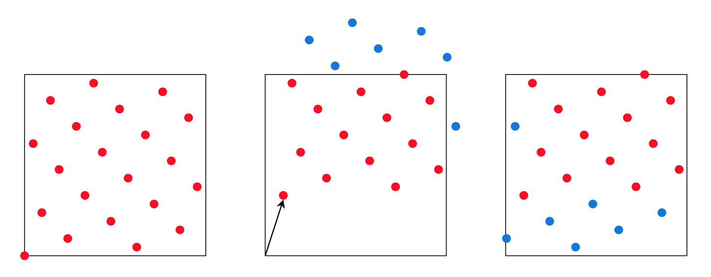
Fig. 64 Applying a $(1/10,1/3)$-shift to a 21-point Fibonacci lattice in two dimensions. Take the original lattice (left), apply a random shift (middle) and wrap the points back onto the unit square (right).

The lattice points given in (53) can be randomized by adding a random shift vector. If $\mathrm{\Delta }$ is a $d$-dimensional vector of standard normal random variables, we construct the shifted lattice points as

$${\mathit{t}}_n=\{\frac{n\mathit{z}}{N}+\mathrm{\Delta }\}.$$

This procedure is illustrated in Fig. 64. Note that the first untransformed point in the sequence will be ${\mathit{t}}^{(0)}=(0,0,\dots ,0)$.

For the lattice points to be practically useful, we would like to transform the lattice rule into a lattice sequence, that allows us to generate well-distributed points for an arbitrary number of points $N$. To this end, Eq. (53) is adapted to

$${\mathit{t}}^{(i)}=\{{\varphi }_b(i)\mathit{z}\},$$

where ${\varphi }_b(i)$ denotes the so-called radical inverse function in base $b$ (usually, $b=2$). This function transforms a number $i=(\dots i_2{i}_1{)}_b$ in its base-$b$ representation to ${\varphi }_b(i)=(0.i_1{i}_2\dots {)}_b$. Note that the radical inverse function agrees with the original formulation when $N=b^m$ for any $m\ge 0$.

Digital nets and sequences

Digital nets and sequences were introduced by Niederreiter, building upon earlier work by Sobol and Faure [Nie87]. In the digital construction scheme, a sequence in $d$ dimensions generates points ${\mathit{t}}^{(i)}=(t_{i,0},t_{i,1},\dots ,t_{i,d})$, where the $j$th component $t_{i,j}$ is constructed as follows:

1. Write $i$ in its base-$b$ representation, i.e.,

$$i=(\dots i_3{i}_2{i}_1{)}_b=i_1+i_{2}b+i_3{b}^2+\dots$$

2. Compute the matrix-vector product

$$\begin{array}{r}\left(\begin{array}{c}{y}_1\\ y_2\\ y_3\\ ⋮\end{array}\right)=C_j\left(\begin{array}{c}{i}_1\\ i_2\\ i_3\\ ⋮\end{array}\right)\end{array}$$

where all additions and multiplications are performed in base $b$.

3. Set the $j$th component of the $i$th points to

$$t_j^{(i)}=\frac{y_1}{b}+\frac{y_2}{b^2}+\frac{y_3}{b^3}+\dots =(0.y_1{y}_2{y}_3\dots {)}_b$$

The matrices $C_j$, $j=1,2,\dots ,d$ are known as generating matrices, see [DP10].

We can encode the generating matrices as an integer matrix as follows. The number of rows in the matrix determines the maximum dimension of the lattice rule. The number of columns in the matrix determines the log2 of the maximum number of points. An integer on the $j$th row and $m$th column encodes the $m$th column of the $j$th generating matrix $C_j$. Since the $m$th column of $C_j$ is a collection of 0’s and 1’s, it can be represented as an integer with $t$ bits, where $t$ is the number of rows in the $j$th generating matrix $C_j$. By default, the encoding assumes the integers are stored with least significant bit first (LSB), so that the first integer on the $j$th row is 1. This LSB representation has two advantages.

• The integers can be reused if the number of bits $t$ in the representation changes.

• It generally leads to smaller, human-readable numbers in the first few entries.

The Sobol sequence is a particularly famous example of a digital net [Sobol67]. A computer implementation of a Sobol sequence generator in Fortran 77 was given by Bratley and Fox [BF88] as Algorithm 659. This implementation allowed points of up to 40 dimensions. It was extended by Joe and Kuo to allow up to 1111 dimensions in [JK03] and up to 21201 dimensions in [JK08]. In the Dakota implementation of the algorithm outlined above, we use the iterative construction from Antonov and Saleev [AS79], that generates the points in Gray code ordering. Knowing the current point with (Gray code) index $n$, the next point with index $n+1$ is obtained by XOR’ing the current point with the $k$th column of the $j$th generating matrix, i.e.,

$$t_j^{(n+1)}=t_j^{(n)}\oplus C_{j,k}$$

where $k$ is the rightmost zero-bit of $n$ (the position of the bit that will change from index $n$ to $n+1$ in Gray code).

The digital net points can be randomized by adding a digital shift vector. If $\mathrm{\Delta }$ is a $d$-dimensional vector of standard normal random variables, we construct the shifted lattice points as ${\mathit{t}}^{(i)}\otimes \mathrm{\Delta }$, where $\otimes$ is the element-wise $b$-ary addition (or XOR) operator, see [DP10]. Note that the first untransformed point in the sequence will be ${\mathit{t}}^{(0)}=(0,0,\dots ,0)$.

Ideally, the digital net should preserve the structure of the points after randomization. This can be achieved by scrambling the digital net. Scrambling can also improve the rate of convergence of a method that uses these scrambled points to compute the mean of the model response. Owen’s scrambling [Owe98] is the most well-known scrambling technique. A particular variant is linear matrix scrambling, see [Matouvsek98], which is implemented in Dakota. In linear matrix scrambling, we left-multiply each generating matrix with a lower-triangular random scramble matrix with 1s on the diagonal, i.e.,

1 0 0 0 0
x 1 0 0 0
x x 1 0 0
x x x 1 0
x x x x 1

Finally, for the digital net points to be practically useful, we would like to transform the digital net into a digital sequence, that allows us to generate well-distributed points for an arbitrary number of points $N$. One way to do this is to generate the points in Gray code ordering, as discussed above.