Anatomy of a Dakota Study
A Dakota study is described by an input file made of six blocks: environment, method, model, variables, interface and responses. Each block has one job, and together they describe what Dakota should do and how to run your simulation.
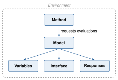
Fig. 4 How the six blocks of a Dakota study relate.
The relationship can be summed up in one sentence: in each iteration of its algorithm, a method requests a variables-to-responses mapping from its model, which the model fulfills through an interface.
This page describes each block, using Rosenbrock’s function as the example throughout.
The example: Rosenbrock
Rosenbrock’s function is a classic test problem for optimization methods, and
Dakota’s examples use it throughout. It has two inputs, x1 and x2, and
one output, f:
The examples on this page vary x1 and x2 between -2 and 2. Over that
range, the function has a single minimum, f = 0 at
(x1, x2) = (1, 1), at the bottom of a long, curved valley. That valley
makes it a useful test:
it is easy to find but hard to follow to its lowest point. Rosenbrock’s
function is built into Dakota, so you can run the examples on this page without
writing any code (except the analysis-driver example under Interface). For
plots of the function, see Rosenbrock Test Problem.
Two formats, one structure
Every block is a tree of keywords. A block contains keywords, and each keyword
can have a value, child keywords, or both. For example, the variables block
below contains the keyword continuous_design, whose value is 2 (the number
of variables), and whose child keywords give the bounds and names of the two
variables.
You can write this tree in either of Dakota’s two input formats. Here is the same variables block in both:
JSON format
{
  "variables": [
    {
      "continuous_design": {
        "count": 2,
        "descriptors": ["x1", "x2"],
        "lower_bounds": [-2.0, -2.0],
        "upper_bounds": [2.0, 2.0]
      }
    }
  ]
}
Freeform format
variables
  continuous_design = 2
    lower_bounds     -2.0     -2.0
    upper_bounds      2.0      2.0
    descriptors       'x1'     'x2'
The JSON format adds a little structure the freeform format leaves implicit.
A keyword’s own value goes in a child field, such as count above, and some
choices are wrapped in a group key, such as gradient_type in the responses
block. See Argument keys and Group keys.
Note
Both formats are fully supported and describe the same study. The
JSON format is easy for scripts and tools to generate
and check. The freeform format is
compact to write by hand. To convert a freeform file to JSON, run
dakota_parser <file> --json.
You run a study in either format the same way:
dakota -json study.json
dakota -i study.in
The rest of this page shows each example in both formats. Choose a tab, and every example on the page switches to that format.
Environment
The environment block holds settings for the whole study, such as which output
files Dakota writes. It’s optional, and a study has at most one. In advanced
studies that combine several methods, it also says which method runs first
(top_method_pointer).
This environment block writes a tabular data file with one row per evaluation, a results file, and a restart file with a chosen name:
{
  "environment": {
    "results_output": {
      "results_output_file": "rosen_multidim_results"
    },
    "tabular_data": {
      "tabular_data_file": "rosen_multidim.dat"
    },
    "write_restart": "rosen_multidim.rst"
  }
}
environment
  tabular_data
    tabular_data_file = 'rosen_multidim.dat'
  results_output
    results_output_file = 'rosen_multidim_results'
  write_restart = 'rosen_multidim.rst'
Learn more: Dakota Output, environment keywords.
Method
The method block chooses the algorithm Dakota runs and its settings. A study needs at least one. Advanced studies can combine several.
This method block asks for a grid of points, dividing the range of each variable into eight intervals. That gives nine values of each variable and 9 × 9 = 81 evaluations:
{
  "method": [
    {
      "multidim_parameter_study": {
        "partitions": [8, 8]
      }
    }
  ]
}
method
  multidim_parameter_study
    partitions = 8 8
To run a different kind of study on the same problem, change the method
block, for example to sampling for uncertainty quantification
or optpp_q_newton for optimization. The Variables and Responses
sections below show both.
Learn more: Study Types, method keywords.
Model
The model block connects a method to the variables, interface and responses
it uses. In a simple study like this one, the model is single and the
block is optional: if you leave it out, Dakota creates a single model for you.
{
  "model": [
    {
      "single": {}
    }
  ]
}
model
  single
Studies that use surrogates, nested studies, or several fidelities of a simulation use more than one model block.
Variables
The variables block defines the parameters Dakota varies, with their bounds or
probability distributions. A study needs at least one. Here, x1 and x2
are continuous design variables, each between -2 and 2:
{
  "variables": [
    {
      "continuous_design": {
        "count": 2,
        "descriptors": ["x1", "x2"],
        "lower_bounds": [-2.0, -2.0],
        "upper_bounds": [2.0, 2.0]
      }
    }
  ]
}
variables
  continuous_design = 2
    lower_bounds     -2.0     -2.0
    upper_bounds      2.0      2.0
    descriptors       'x1'     'x2'
Variables are classified by what they represent, and the kind of variable decides which methods can use it:
Kind |
Represents |
Typically used by |
|---|---|---|
Values you control, such as dimensions or settings |
Optimization, calibration, parameter studies |
|
Aleatory uncertain |
Inherent randomness, described by probability distributions |
Uncertainty quantification, sensitivity analysis |
Epistemic uncertain |
Lack of knowledge, often described by intervals |
Epistemic uncertainty quantification |
Fixed settings, such as solver tolerances or mesh resolution |
Held fixed by most methods; parameter studies can vary them |
Each kind can be continuous or discrete, and discrete variables can take integer, real or string values.
The same Rosenbrock problem can be studied with uncertain inputs instead. Here
x1 and x2 are uniformly distributed on the same range, and the method
block changes to sampling:
{
  "method": [
    {
      "sampling": {
        "sample_type": {
          "lhs": true
        },
        "samples": 100,
        "seed": 1234
      }
    }
  ],
  "variables": [
    {
      "uniform_uncertain": {
        "count": 2,
        "descriptors": ["x1", "x2"],
        "lower_bounds": [-2.0, -2.0],
        "upper_bounds": [2.0, 2.0]
      }
    }
  ]
}
method
  sampling
    sample_type lhs
    samples = 100
    seed = 1234

variables
  uniform_uncertain = 2
    lower_bounds     -2.0     -2.0
    upper_bounds      2.0      2.0
    descriptors       'x1'     'x2'
Interface
The interface block tells Dakota how to run each evaluation: what to call, and how to exchange data with it. A study needs at least one.
A built-in test function. Rosenbrock’s function is built into Dakota, so
this example needs no external code. The direct keyword calls it inside
Dakota:
{
  "interface": [
    {
      "analysis_drivers": {
        "drivers": ["rosenbrock"],
        "interface_type": {
          "direct": {}
        }
      }
    }
  ]
}
interface
  analysis_drivers = 'rosenbrock'
    direct
Your own code, through an analysis driver. To run your own simulation,
you name an analysis driver, a program Dakota runs once per
evaluation. With fork, Dakota starts it as a separate process and
exchanges parameter and result values with it through files:
{
  "interface": [
    {
      "analysis_drivers": {
        "drivers": ["python3 driver.py"],
        "interface_type": {
          "fork": {}
        }
      }
    }
  ]
}
interface
  analysis_drivers = 'python3 driver.py'
    fork
Nothing else in the study changes: the method, variables and responses are the same whether Rosenbrock’s function is built in or comes from your own code. You’ll build and run one in Tutorial: Your First Dakota Study, and Connecting Your Code: The Analysis Driver explains them in depth.
Learn more: Interfaces, interface keywords.
Responses
The responses block describes the responses your simulation returns, and whether derivatives are available. A study needs at least one.
The kind of response matches the kind of study:
objective_functions: quantities to minimize or maximize, for optimization;calibration_terms: differences from data, for calibration;response_functions: general outputs, for parameter studies, sensitivity analysis and uncertainty quantification.
The parameter study uses one response function and needs no derivatives:
{
  "responses": [
    {
      "gradient_type": {
        "no_gradients": true
      },
      "hessian_type": {
        "no_hessians": true
      },
      "response_type": {
        "response_functions": {
          "count": 1
        }
      }
    }
  ]
}
responses
  response_functions = 1
  no_gradients
  no_hessians
To optimize Rosenbrock’s function instead, the method changes to a
gradient-based optimizer, and the responses block declares one objective
function. numerical_gradients tells Dakota to estimate gradients itself,
by finite differences, so your code doesn’t have to provide them:
{
  "method": [
    {
      "optpp_q_newton": {
        "convergence_tolerance": 0.0001
      }
    }
  ],
  "responses": [
    {
      "gradient_type": {
        "numerical_gradients": {}
      },
      "hessian_type": {
        "no_hessians": true
      },
      "response_type": {
        "objective_functions": {
          "count": 1
        }
      }
    }
  ]
}
method
  optpp_q_newton
    convergence_tolerance = 1.0e-4

responses
  objective_functions = 1
  numerical_gradients
  no_hessians
A gradient-based optimizer also needs a starting point, which you set with
initial_point in the variables block. Optimization studies can also
declare constraints in the responses block.
How information flows
When you run a study, Dakota reads the input file and sets up the blocks. The method then asks the model for one evaluation after another. For each one, the model maps the variable values through the interface to response values, and returns them to the method. As the study runs, Dakota writes its progress to the console and records each evaluation in the tabular data file and the restart file.
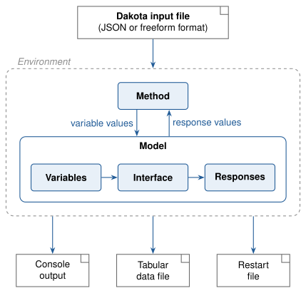
Fig. 5 How information moves through a Dakota study.
The complete input file
Put together, the blocks make a complete study: an 81-point parameter study of Rosenbrock’s function.
{
  "environment": {
    "tabular_data": {
      "tabular_data_file": "rosen_multidim.dat"
    }
  },
  "method": [
    {
      "multidim_parameter_study": {
        "partitions": [8, 8]
      }
    }
  ],
  "model": [
    {
      "single": {}
    }
  ],
  "variables": [
    {
      "continuous_design": {
        "count": 2,
        "descriptors": ["x1", "x2"],
        "lower_bounds": [-2.0, -2.0],
        "upper_bounds": [2.0, 2.0]
      }
    }
  ],
  "interface": [
    {
      "analysis_drivers": {
        "drivers": ["rosenbrock"],
        "interface_type": {
          "direct": {}
        }
      }
    }
  ],
  "responses": [
    {
      "gradient_type": {
        "no_gradients": true
      },
      "hessian_type": {
        "no_hessians": true
      },
      "response_type": {
        "response_functions": {
          "count": 1
        }
      }
    }
  ]
}
# Dakota Input File: rosen_multidim.in
# Usage:
#   dakota -i rosen_multidim.in -o rosen_multidim.out > rosen_multidim.stdout

environment
  tabular_data
    tabular_data_file = 'rosen_multidim.dat'

method
  multidim_parameter_study
    partitions = 8 8

model
  single

variables
  continuous_design = 2
    lower_bounds     -2.0     -2.0
    upper_bounds      2.0      2.0
    descriptors       'x1'     "x2"

interface
  analysis_drivers = 'rosenbrock'
    direct

responses
  response_functions = 1
  no_gradients
  no_hessians
To see the results of this study, read Rosenbrock Test Problem, or run it yourself in Tutorial: Your First Dakota Study.